Chapter 8:
Frequent Modulations

In this chapter we’re going to look at some common (and less common) ways to modulate one oscillating signal by another, mostly at audio rates. This includes amplitude and ring modulation (AM and RM), frequency and phase modulation (FM and PM), and some interesting extensions to them. These methods are relatively simple and often computationally economical ways to generate interesting waveforms and spectral richness with smooth and continuous evolutions. Sometimes these subjects, and FM in particular, have an air of mystique or impenetrability. We hope to show not only how they are really quite approachable, but also through the flexible capabilities of gen~, how we can go beyond traditions to explore new and unusual algorithms and structures.

Amplitude modulation (AM) and Ring Modulation (RM)

One of the simplest things we can do with a signal is make it quieter, which means reducing its amplitude, which means multiplying every signal value by some number less than one. If the multiplier is a signal that varies over time, we can call it a “modulator”, as it is modulating the amplitude of our original signal (which we call the “carrier”). This is known as amplitude modulation (or AM for short). This is what we are doing when we repeatedly envelope a sound, for example. An envelope typically runs from 0.0 (silence) to 1.0 (full amplitude) and back. That is, the modulator is unipolar.

Let’s start with a simple bipolar sine wave at 100Hz (using a cycle 200 operator) as the carrier: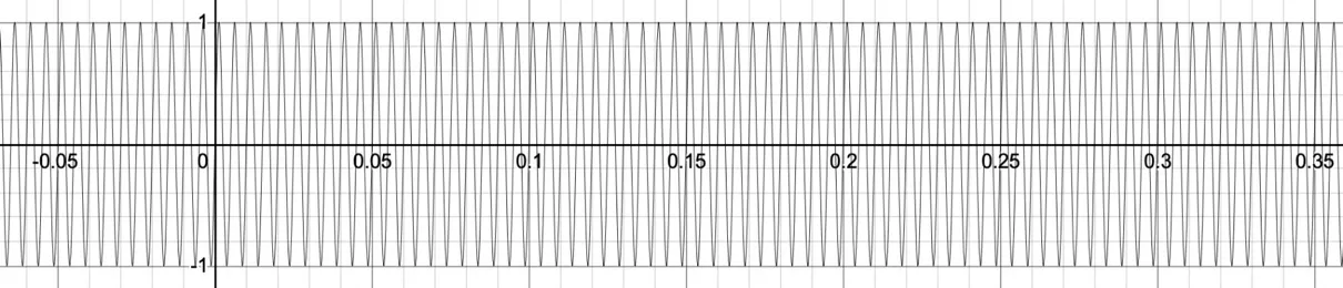

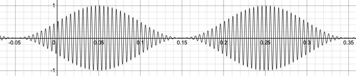
…and for the modulator, a unipolar sine wave at 5 Hz. We can make a cycle 5 operator unipolar by sending it through a scale -1 1 0 1 operator[73]:

Then, multiplying these two signals produces our AM result:

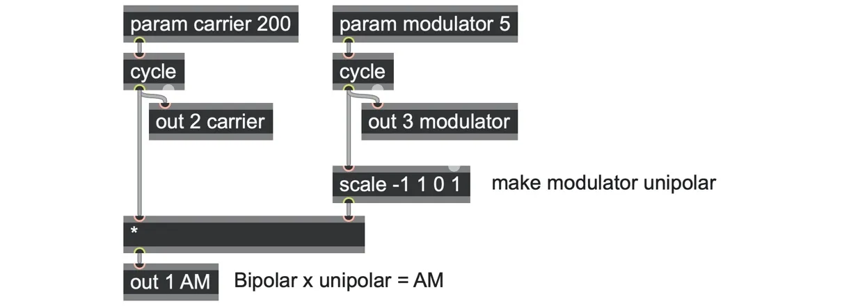
AM.maxpat

With the modulator frequency at 5Hz, the effect is a series of distinct sound events, like primitive notes. If you speed the modulator up to about 15Hz, it turns into a quite intense rhythmic tremolo effect. We’ll look at reducing the intensity shortly, but first, try pushing the modulator frequency gradually upwards. At somewhere around 25-40Hz, the rhythmic sensation transforms into a kind of “fused” complex timbre. Above 40Hz, as you slowly keep rising, you may start to hear other tones appear, at certain points sounding like chords. With the carrier frequency at 600Hz, try modulator frequencies at 200Hz or 300Hz, for example. It’s quite remarkable that with a single parameter we can evoke so many musical elements: note events, trill/tremolo, timbre, and chords.[74]

Sidebands

To understand what’s happening here, we can have a look at the spectrum. Here is the carrier, a pure sine wave at 800Hz:

Here is the modulator, a pure sine wave at 200Hz:

And here’s the AM output, showing a peak at 800Hz, but also at 600Hz and 1000Hz:

Regardless of how we change the carrier and modulator frequency params, there’s a copy of the carrier frequency present, a tone above, and a tone below it whose spacing increases as the modulator frequency increases. In fact, for sine waves, the frequencies of these “sideband” tones can be precisely predicted as:

CarrierHz + ModulatorHz

CarrierHz — ModulatorHz

Notice that the calculation can result in negative sideband frequencies. For example, if the carrier is 100Hz, and the modulator is 300Hz, then there will be sidebands at 400Hz and -200Hz. We can’t hear any difference between positive and negative frequencies by themselves, but it can lead to waveforms interfering and cancelling each other out in unexpected ways. We’ll also see this also for the other kinds of modulation in this chapter.

Ring modulation

Let’s go back to the tremolo at 15Hz and reduce its depth. If we could make our modulator run between, say, 0.8 and 1.0, then the modulation depth would be decreased, and the tremolo effect would be more subtle.

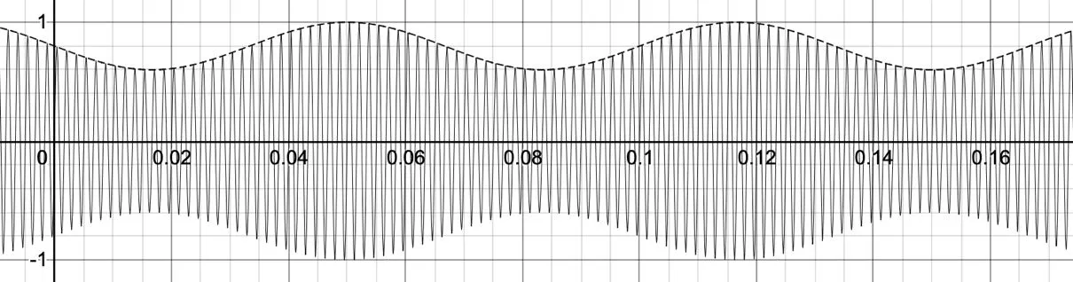
We can control this depth by modifying our scale operator to set the minimum value with a param low and thus map our original modulator’s range (-1.0 to 1.0) to our desired range (param low to 1.0).

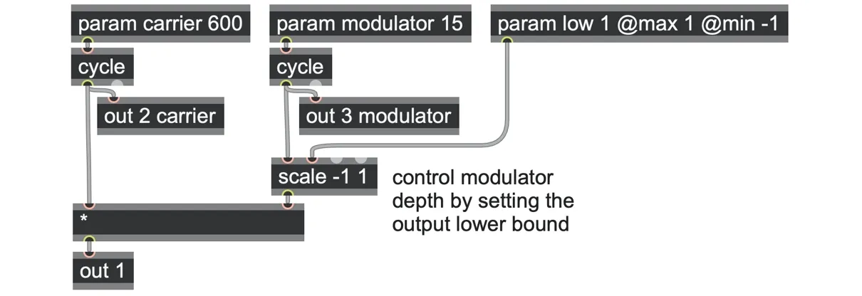
AM-depth.maxpat

Initially, there is no tremolo effect at all, but as we bring the param low from 1.0 down towards zero, the depth of the tremolo intensifies.

Turn the modulator frequency back up to 200Hz again. Now slowly push the param low further down all the way to -1.0 while watching the spectrum. You will see the “central lobe” at the carrier’s 600Hz fade away toward zero, while only the sideband lobes at 400Hz and 800Hz remain (now slightly louder. At the point where param low equals -1.0, the scale operator is actually doing nothing at all: we are simply multiplying two bipolar oscillators, which is called ring modulation[75] (RM):

Here are some observations.

• Ring modulation (RM) is just a multiplication of two bipolar signals

• Amplitude modulation (AM) is a multiplication of a bipolar with a unipolar signal

• Amplitude modulation has the same sidebands as RM, mixed with the original carrier

• Amplitude modulation looks like a mix between RM and the original carrier

That last observation is mathematically correct, in fact. Call the bipolar carrier “C” and the bipolar modulator “M,” then we can simply say that

RM = C * M

and

AM = C * ((M * 0.5) + 0.5)

Note that ((M * 0.5) + 0.5) is the equivalent of a scale -1 1 0 1 operator.

Doing a little rearranging:

AM = (C * M * 0.5) + (C * 0.5)

AM = (RM * 0.5) + (C * 0.5) (because RM = C * M)

AM = (RM + C) * 0.5

That last expression is an exact average. So, we could actually express our blend from C to AM to RM as a more intuitive linear mix.

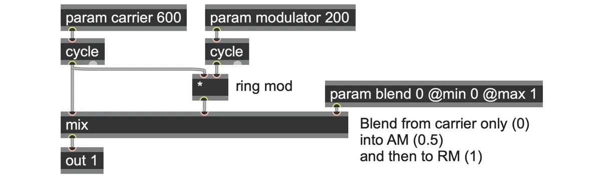
AMRM.maxpat

Beyond sinusoids

What happens if we start using waveforms other than sine waves for our carrier and modulator? The Fourier theorem says that any complex periodic signal can be described as simply a mixture (a sum) of plain old sine waves at different frequencies, amplitudes, and phases. What the spectroscope is showing us is an approximation of that mixture of sine waves. But most interesting waveforms need quite a large number of sine wave components, and since every single pairing of these between carrier and modulator creates two more sidebands, it can easily end up becoming a huge number of sidebands, and it can get complex very quickly. Still, if the carrier and modulator are harmonically related, and their component sine waves are harmonics, then many of those sidebands might end up overlapping such that the final waveform is likely to be harmonic too.

Frequency modulation (FM) and phase modulation (PM)

In the last section, we saw how speeding up a tremolo effect turns into the spectral effects of amplitude and ring modulation. In a similar way, speeding up a vibrato effect can open up the strange worlds of frequency modulation (FM) and phase modulation (PM).[76] As we’ll see in this section, these two techniques are very similar to each other and have the same results in many cases.

Let’s keep things simple by starting with sine waves again. This time, we’re going to build a sine wave oscillator from a phasor operator rather than using the cycle operator. The main reason for this is that we’re going to need to manipulate the sine wave oscillator at a finer level than a cycle operator affords.

Making this change will also make it easier to use waveforms other than sine waves later on as well. Here is our basic sine oscillator:

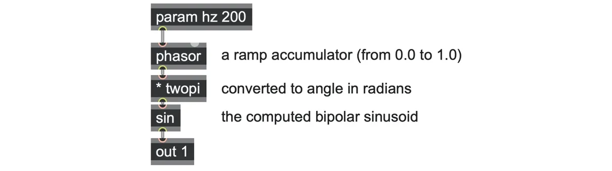
Sine.maxpat

The simplest PM and FM circuits use two of these oscillators — one being the “carrier” and the other the “modulator.” Here is the main difference between PM and FM

• In PM, the modulator is added to the angular phase before it enters the carrier’s sin operator.

• In FM, the modulator is scaled to a value in Hz and added to the frequency before it enters the carrier’s phasor operator.

In addition, in both cases, the amount of modulation added is multiplied by a parameter called the modulation index (or sometimes called the depth).

Here are the two circuits side by side, with PM on the left and FM on the right. As you can see, the difference between these two circuits is fairly minimal. The main difference is whether we are modulating the phase, or the rate of change of phase.[77]

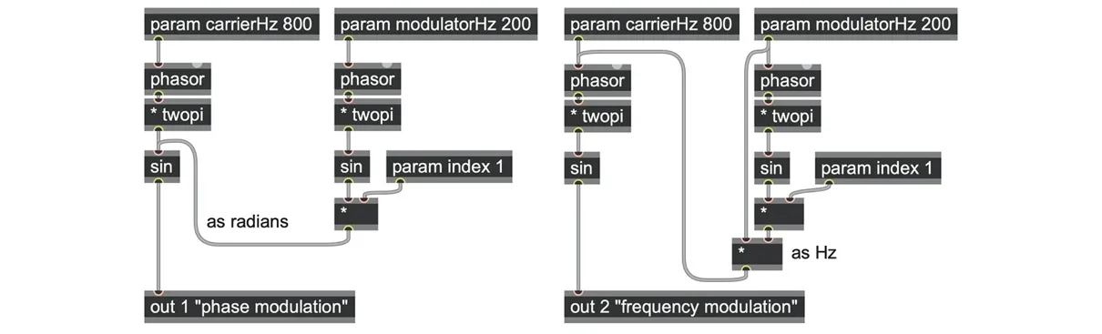
FMPM.maxpat

Sidebands

As it turns out, the spectra coming out of these two circuits are identical, regardless of what the parameters are. The waveforms also look virtually the same, however their relative phases may be different. And as long as the param index is fairly low, the spectra also look a bit similar to amplitude modulation, with a peak at the carrier, and symmetric sidebands above and below:

But for FM and PM, there are a lot more sidebands—and so the timbres and spectra of FM and PM are much more complex. For a carrier frequency of “C” and a modulator frequency of “M,” the output frequencies are at the carrier C followed by pairs of sidebands at C+M and C-M just like AM/RM, but also at C+2M and C-2M, C+3M and C-3M, and so on. More generally:

CarrierHz + k * ModulatorHz

CarrierHz - k * ModulatorHz

Where k indicates the whole numbers 1, 2, 3, etc. For example, with a carrier at 1600Hz and modulator at 100Hz, the spectrum shows a strong central peak at 1600 Hz, sidebands above at 1700Hz, 1800Hz, 1900Hz, etc., and symmetric sidebands below at 1500Hz, 1400Hz, 1300Hz, etc.

The intensity of each of these pairs of sidebands depends on the modulation index in a complex way[78], but it is generally the case that increasing the index will increase the number of sidebands heard, with their intensity spreading out from the carrier frequency as the index increases, resulting in brighter and more complex sounds.

The following spectra below show the spectrum with param index at 1, 4, and 10, respectively.

Therefore, many implementations use an envelope signal to control this modulation index and thus shape the PM or FM spectrum into an expressive event, such as rising quickly to a bright sound and then decaying more slowly to a duller sound, a timbral profile common to many musical instruments. We can extend our patch to support this by multiplying the param index with an in 1 operator for the modulation signal input (and feeding an envelope of choice into that input). And while we are at it, why not also multiply the output with a related amplitude envelope to control the overall loudness of the event?

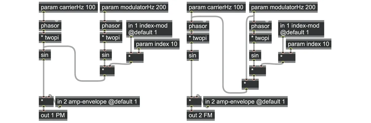
FMPM-enveloped.maxpat - on the left is the PM patch, on the right is the FM patch.

Frequency ratios and harmonicity

If you play around with the carrier and modulator frequencies in the FMPM.maxpat or FMPM-enveloped.maxpat patches, you may notice that some combinations of frequencies are more clangorous, metallic, bell-like, or enharmonic than others. Since sidebands appear at C + k*M, where k is some positive or negative whole number, it makes sense that the sidebands will form a more harmonic alignment with the carrier when the ratio of the modulator and carrier frequencies is made of simple whole numbers, such as 1:2, 1:5, 4:3, etc. This ratio is sometimes called the “harmonicity ratio.” For example, when the modulator frequency is twice the carrier frequency (a ratio of 2:1), the resulting spectrum will contain only odd harmonics, much like a square wave.

But whole number ratios are not the only ones that can create harmonic partials. As John Chowning himself put it (on a post on the Cycling ’74 forum[79]), it is better to think of there being a fundamental frequency (or pitch) control and to set carrier and modulator as multiples of that core frequency. That way, the spectral shape of the sound stays consistent as the core frequency (or pitch) control changes, and the sound will be harmonic if the carrier and modulator multipliers form a simple ratio (such as 3:2, 2:3, 3:4, 4:3, etc.). It is this ratio that defines the harmonicity. Following Chowning’s recommendation, we can modify our patch to include separate fundamental frequency, as well as carrier and modulator multiplier parameters from this point onward.

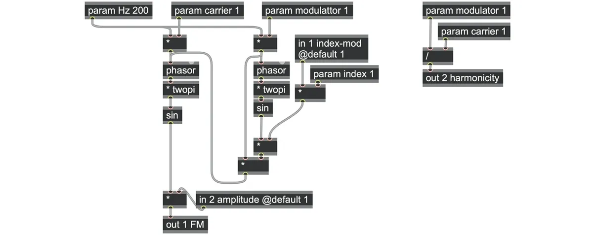
FMPM-harmonicity.maxpat (here showing the PM implementation).

It’s also highly recommended to try ratios that are almost but not quite whole ratios, such as 1 : 3.01, as these slightly detuned frequencies will produce undulating “beating” variations that deepen the timbre. You could also add a tiny amount of noise (or one of the smooth random generators from Chapter 4 to the modulator frequency!

For some low carrier and high modulator parameter combinations, some of the sidebands will go “below zero.” For example, if C=5Hz and M=10Hz, even the first sideband of C-kM is at -5V, the next at -15Hz, the next at -25Hz, etc. These sidebands don’t disappear — they simply mirror around the zero Hz line and rise back up with their phase inverted (their waveform runs backward). For a symmetric waveform such as a sine wave, this is no different than an imperceptible phase-shift. While those negative frequency sidebands can add to the characteristically clangorous sound of FM and PM, something interesting happens when the harmonicity ratio is simple: the folded negative sidebands may line up with the regular sidebands, resulting in a harmonic sound.

Combinations (FM algorithms and beyond)

So far, we’ve only looked at patches with a single modulator oscillator feeding a single carrier oscillator. Historic hardware phase modulation synthesizers such as the Yamaha DX7 included more oscillators with a variety of “algorithms” to choose from, where the term algorithm really meant pre-defined configurations of a handful of ways of wiring these oscillators together.

In this section, we’ll delve deeper into these as well as several other ways of combining oscillators through mutual modulation. This is another example of where gen~ offers great freedom: rather than being limited to selecting from pre-defined configurations, we can freely rearrange signal structures and explore new ones by inserting different processes between them, including single-sample feedback loops.

To keep things simple, we’ll focus mostly on phase modulation, as it is slightly easier to construct and maintain pitch stability. Many of the patches include FM implementations, too.

Parallel carriers and parallel modulators

Parallel carriers refers to the technique of sending a modulation signal into more than one carrier and mixing the results together. Adding more carriers can be a relatively controllable way of producing coherent formants.

The following example blends two carriers with a linear mix operator.

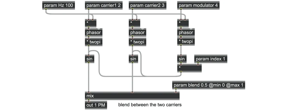
FMPM-parallel-carriers.maxpat

Similarly, we can easily combine multiple modulators together — here are two modulators routed into a single carrier.

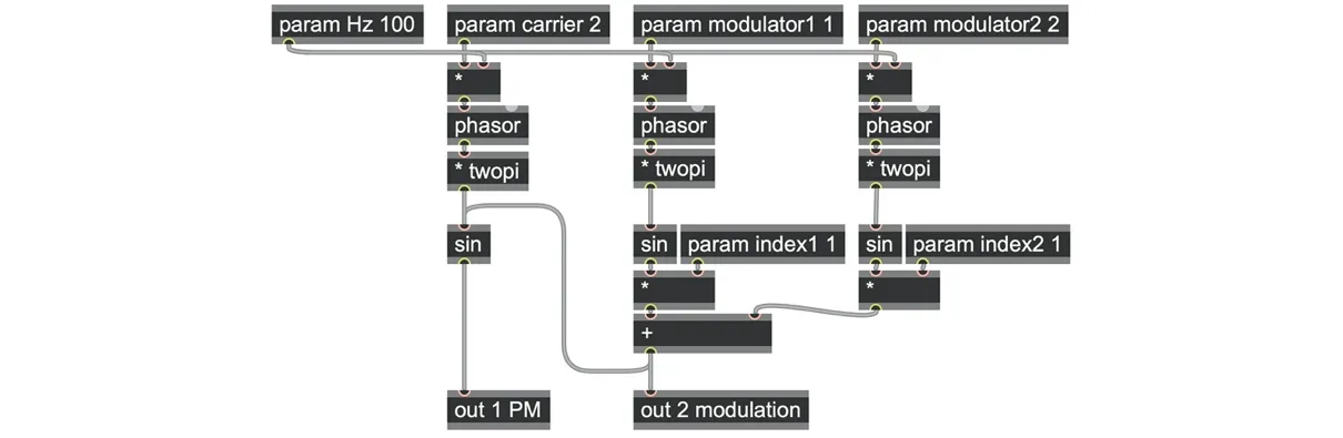
FMPM-parallel-modulators.maxpat

The FMPM-parallel-modulators.maxpat patch also shows the FM equivalent (they sound the same). For more movement, try carrier to modulator ratios that are slightly detuned from simple fractions, like 2:3.01.

Beyond sinusoidal modulators

We can use these patches to understand what PM and FM mean for more complex waveforms. Take a look at the FMPM-parallel-modulators.maxpat patch again. The modulation signal that goes from the + operator to the sin operator is just one signal (we can take a look at it from out 2), which has a waveform made from two sine waves added together. The PM or FM spectrum this produces creates a whole set of sidebands for each of those two sine waves.

From this, we can extrapolate that any waveform made up of a more complex combination of component sine waves will create a whole set of sidebands for each sine wave component. And, since the Fourier theorem shows that any periodic waveform can be created from a collection of sine waves, we now have a better idea of what to expect from more complex modulator waveforms.

One quick observation we can make is to note how quickly waveforms with significant high harmonics can produce sidebands at extremely high frequencies, which as we shall see can cause aliasing distortion. Accordingly, many PM and FM implementations restrict their oscillator waveforms to sine waves, waveforms whose harmonics fall quickly, such as triangle waves, or waveforms that can be band-limited to only include lower harmonics. We’ll return to this later with respect to band-limiting signals.

Moving beyond basic sinusoidal modulators, we also start to hear differences between PM and FM. The FMPM-blending.maxpat patch demonstrates this using a triangle wave modulator (and also shows how we can blend smoothly between PM and FM using an equal power mixer).

Why does a non-sinusoidal waveform sound different for PM and FM? Remember that when we hear a sound, our sense of its pitch or frequency doesn’t come from the size of the wave, but from how quickly it oscillates, that is, its rate of change (or, in mathematical terms, its derivative).

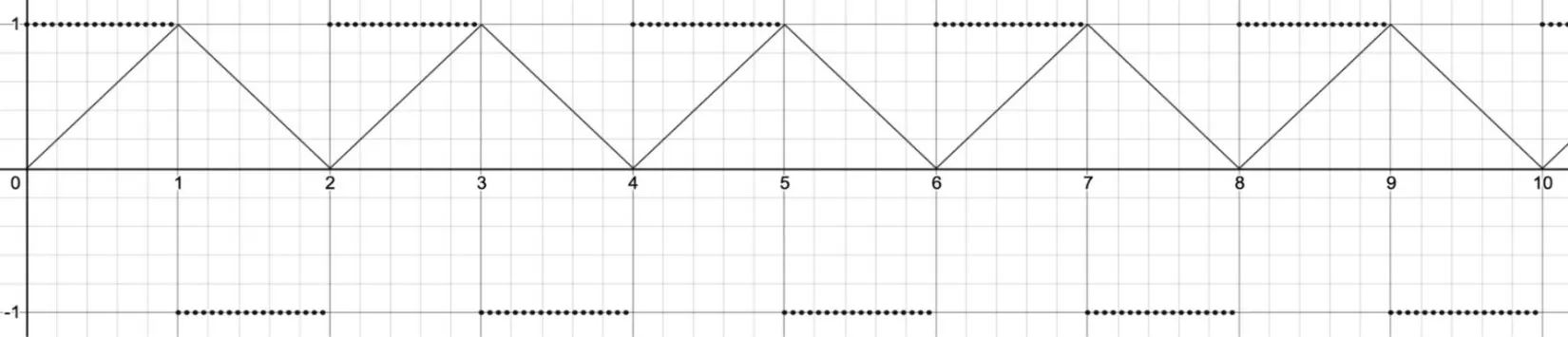
Let’s keep things simple by choosing a slow triangle wave as a modulator (solid line in the graph above). The rate of change of a triangle wave is a positive constant when the triangle is rising and a negative constant when the triangle is falling; that is, the rate of change of a triangle wave is a square wave (dotted line above). So if you use a triangle wave modulator in PM, you will alternately hear a high pitch, then a low pitch, and so on. In contrast, with FM, we feed the modulator through a phasor operator first.

You may remember from Chapter 2 how we built the phasor operator from a process of counting, which makes it act like an integrator in mathematical terms: it converts the value at the input into a rising or falling slope at the output (i.e., it converts the input into a rate of change). So, our triangle wave modulator in FM directly produces rates of change of the carrier signal, alternately speeding it up and then slowing it down, which we hear as a rising and falling pitch, like a vibrato.

That’s why the modulator directly shapes the pitch of the output in FM, but it is the modulator’s rate of change (slope or derivative) that shapes the pitch of the output in PM. The reason we couldn’t hear this difference with a simple sine wave modulator is that the rate of change of a sine wave is another sinusoidal wave[80]—this is part of what makes sine waves so special. But once you start using other waveforms, including even simple mixtures of sine waves, the differences become far more obvious.

To take this insight one step further, have a look at the second example in FMPM-blending.maxpat, and you’ll see that even though we are using a skewed triangle wave modulator, both FM and PM sound identical. How? Because we fed the PM modulator through a lowpass filter (which, as we saw in Chapter 6, is a kind of integrator) and the FM modulator through a highpass filter (a kind of differentiator)! That is, FM using a highpass filtered modulation signal is exactly the same as PM using the lowpass filtered modulation signal!

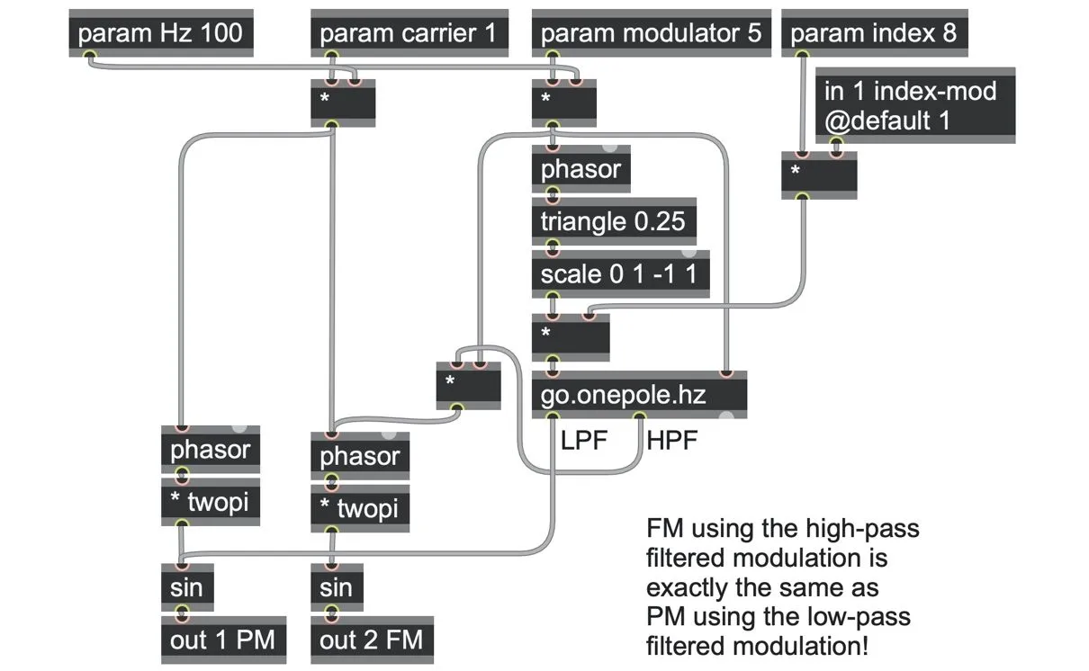
FMPM-blending.maxpat

Modulating modulators: cascade modulators

What if we use another PM or FM signal as our modulator? This is sometimes called series modulation or cascade modulation, as it simply means that our modulator is modulated by another modulator.

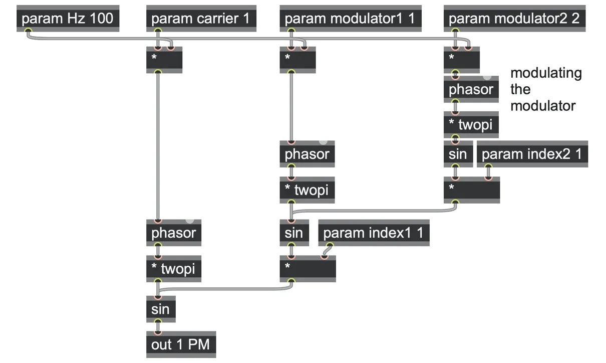
The FMPM-cascade-modulation.maxpat patch shows this PM implementation of cascade modulation, as well as a comparable FM implementation. Unlike simpler configurations, once the modulator’s modulator’s index (here, the param i2) is non-zero, the PM and FM versions respond differently–with the PM version producing comparably brighter spectra.

As with parallel modulators, cascade modulation is equivalent to a single modulator with a more complex and dynamic waveform, but it can achieve this complexity with far fewer oscillators. The timbral spectrum of the sidebands has a slightly recursive quality, as each sideband produced in the second modulator creates a whole set of sidebands in the carrier.

Cascading more modulators increases this recursive complexity.

Feedback modulation

Could we create a cascade of infinite modulators? Actually, this can be done very easily by simply feeding the carrier’s output back through a history operator to become its own modulator.

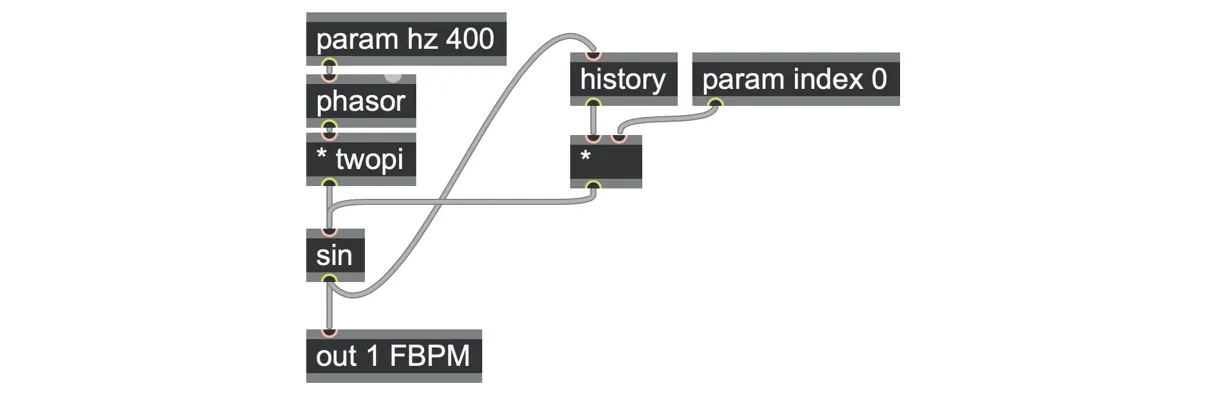
FMPM-feedback.maxpat

With an index parameter of zero, there is no feedback at all, and we hear the pure carrier sine wave. As the index is brought up to 1.0, the sine becomes increasingly skewed toward a rounded saw wave. Turning the index down to -1.0 will skew in the other direction.

Unlike the unusual distribution of often clangorous sidebands in typical multi-operator phase modulation, the sidebands have a more naturalistic exponential distribution with feedback modulation, and they are always harmonic.

But as we increase the index further, you can start to hear distortions appear. The feedback modulation patch is a very basic chaotic iterated system, and these distortions are examples of “hunting” phenomena in the chaos. Keep turning the index parameter up and it will eventually collapse into complete noise. This noise can be handy for a bright “strike” effect if driving the index with an envelope, but it sets in rather quickly.

The original patent for Yamaha’s implementation by Norio Tomisawa[81] added a filter in the feedback loop to lessen the impact of this chaotic behavior; in the patent, this filter was a very simple average with the previous input (a finite impulse response filter), which allows the index to go up to about 2.0 without any chaotic disturbance.

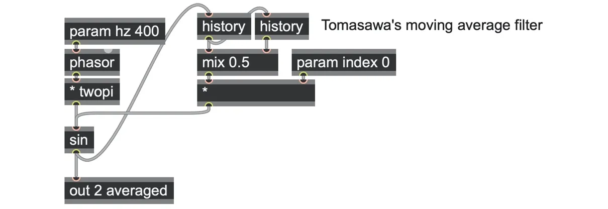
FMPM-feedback.maxpat

If instead we insert a one-pole lowpass filter such as the go.onepole.hz we built in Chapter 6 and tune it to a cutoff frequency somewhere between 200 to 4000Hz, we can push the modulation index much higher. However, as we lower the cutoff frequency, the output waveform becomes more spiky and less saw-like.

^pAs an alternative, we can have the lowpass filter’s cutoff frequency track the same frequency as the carrier, as in the following patch, which results in a very stable output even with a much higher index.

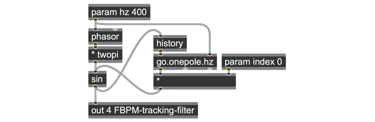
FMPM-feedback.maxpat

Feedback FM modulation can also be implemented in a similar way, but the behavior is rather different, leading to a spikier waveform.

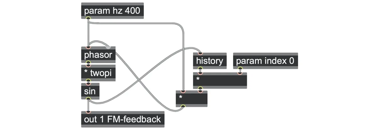
FMPM-feedback.maxpat

Unfortunately, the asymmetry of this waveform in feedback also effectively “detunes” the oscillator. We’ll look at why (and how to fix this) in the next section.

Fixing FM going out of tune

If the modulator signal is not balanced around the zero line, which is to say that the average of the value of the modulation over time is not zero, then that deviation is called a bias or DC offset. Any such DC offset in an FM modulator will be heard as a detuning of the carrier. A tiny amount of very low frequency modulation might be desirable, as slight detuning can add to the warmth or “fatness” of a sound, but beyond this we may likely want to eliminate more significant detuning due to DC. We can suppress it quite effectively using a highpass filter[82] (such as the middle outlet of go.onepole.hz). For example, here’s that solution applied to feedback FM.

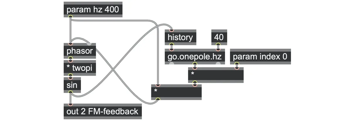
FMPM-feedback.maxpat

In this patch, we made the filter track the same frequency as the modulator, but you could also try using a fixed filter frequency tuned to the threshold of audibility somewhere between 10 to 50Hz. Regardless, it is generally best to place this filter before scaling the modulator by the modulation index so that the effects of envelopes are not filtered away.

Highpass filtering is not usually necessary for PM since a DC offset there leads to a change in phase rather than a change in pitch. But here’s something very curious—if you compare the output and response of the feedback PM patch with the tracking lowpass filter and the feedback FM patch with the tracking highpass filter, they now look remarkably similar

Cross-coupled feedback modulation

So far, our feedback modulation patches have had a single oscillator, but we can also create feedback with two (or more) oscillators, where each acts as a modulator to the other. In this “cross-coupled” feedback, either oscillator can be the output (or both).

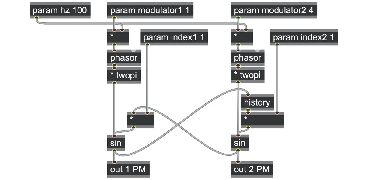
PM-cross-feedback.maxpat

As long as both index parameters are non-zero, this creates a feedback loop through both oscillators. The resulting waveform combines the saw-like spectrum of feedback PM with the complex spectrum of ordinary PM.

As with single-oscillator feedback PM, inserting a lowpass filter in the feedback loops permits much higher index parameters and more elaborate transitions into chaos. In between, it can sometimes jump between bifurcations of harmonics and other very expressive sounds. The feedback filter cutoff has a strong impact on the output spectrum.

For the following patch, we set the filter frequency parameters to be multiples of the modulator frequencies.

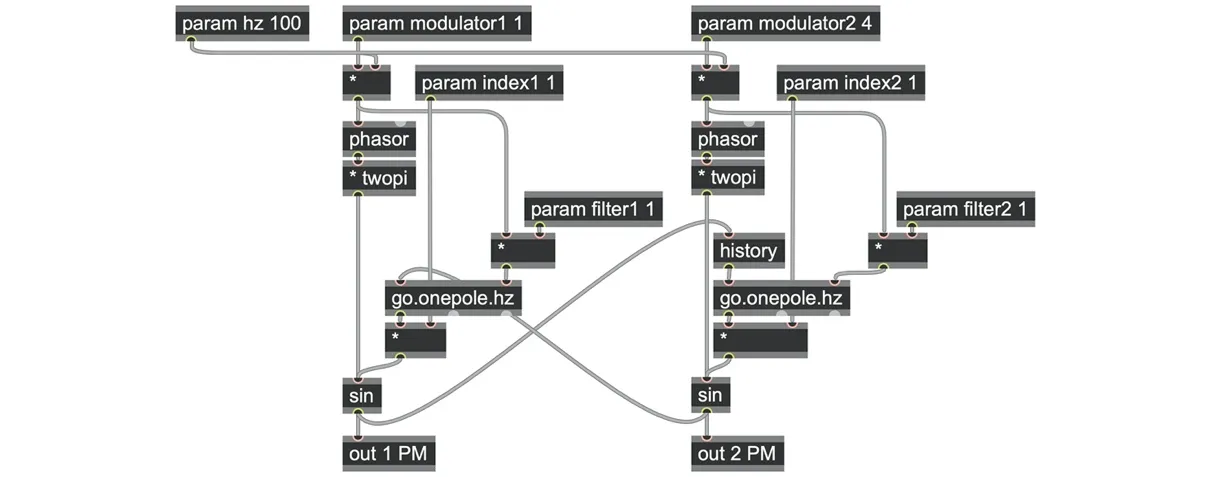
PM-cross-feedback-filtered.maxpat

Try setting the carrier frequencies to slightly detuned from a whole number multiples of each other to hear how this interacts with the beating frequencies.

Or, for something completely different: set one carrier at an audible rate (e.g., 50-100Hz) and high index (e.g., 100-200), and the other at a slow LFO rate (around 1Hz) and low index (around 4) and explore the complex soundscapes that ensue as you move the filter cutoff frequencies between 5Hz and 250Hz. The results can sound remarkably analog and can be surprisingly hard to predict!

Exploring hybrid algorithms

Most of the algorithm structures we have looked at so far are pretty lightweight in computational cost and can easily be extended and combined to involve more oscillators. But with an environment like gen~ why stop there? For example, what happens when we combine parallel, cascade, and feedback structures with other signal processors besides PM and FM, such as AM/RM, waveshaping, or other filters and delays? What happens when we introduce colored noise, chaos, quantized or smooth-stepped signals into these circuits? There’s a huge range of possibilities to explore!

Index amplitude/ring modulation

Actually, we’ve already been doing some of this, more or less. We’ve seen that multiplying the param index with an envelope can create expressive sound events, but there’s no reason to limit yourself to sending envelopes into that in 1 mod-index operator! Try throwing all different kinds of modulations in here, such as LFOs (for a classic ‘wub wub’ sound, see FMPM-lfod.maxpat) and audio-rate oscillators. In fact, if you think about it, inserting an oscillator here is like applying amplitude or ring modulation to the modulator before it modulates the carrier!

Phase modulation: suppressing clicks

You might notice that, with phase modulation, making rapid changes to the modulation index can lead to clicks and distortions in the carrier. This makes sense: any sharp transients or jumps of magnitude in the modulator signal will become sudden jumps of phase of the carrier and cause skips in the output waveform.[84]

For example, in the following graph, the index of modulation (dashed line) is a stepped random signal whose steps cause the modulation signal (thin dotted line) to jump in magnitude. As a result, the phase modulation output (solid line) has skips and breaks in its flow that will be heard as clicks.

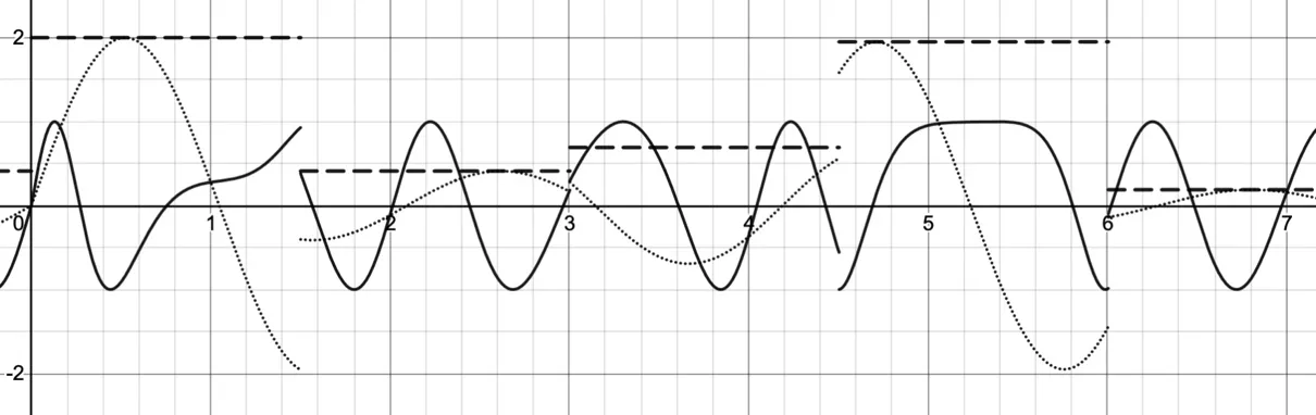
There are a couple of ways we can address this.

One way is to sneak in the index changes by updating it only when the modulator signal is crossing zero (i.e., the very moment at which the index scaling has no effect) using a zero-crossing detector and a latch operator.

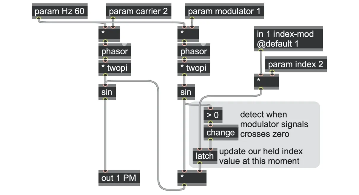
PM-noclicks-latched.maxpat

The technique of introducing a change in parameters at the point where the algorithm is temporarily silenced is one you’ve seen before in this book (for example, where we used it to change a delay time without adding a pitch shift in Chapter 7. For the phase modulation patch above, latching the index when the modulator is near zero, and thus having no effect on the carrier, quite effectively hides the discontinuities (at least, so long as the modulator has no significant DC offset).

An alternate method is to add a slew or lowpass filter to the index parameter before the modulation is added to the carrier to soften any jumps by spreading them out over time. The filter may need to be tuned to fit each application as needed since the more it suppresses clicks, the more it may also limit the brightness of the index modulation itself. In PM-noclicks-filtered.maxpat we chose a series of three stacked one-pole filters at around 500Hz as a reasonable tradeoff.

Waveshaping modulators

Take a closer look at almost any of the patches we’ve explored so far. No matter what we do to create our modulation, you can see that the resulting signal always goes through the sin operator just before the output, which means that the output will always be swinging between -1.0 and 1.0. Compared to creating sounds “additively” by mixing sine waves together, phase modulation and frequency modulation are much cheaper ways to produce a spectrum that is not only complex but also energetically optimal.

Try setting the carrier frequency to zero. Now the perceived pitch is entirely determined by the modulator, and increasing the index parameter creates an effect very much like wave folding or wave shaping.[85] In fact, for phase modulation, that carrier sin operator really is acting as a waveshaper: no matter what crazy modulations we throw at it, it ensures the output is wrapped within the -1.0 to +1.0 range. We could also try different periodic waveshaping functions here instead of a sin operator (such as a triangle, sinh, or fold operator), and we’ll return to this notion when we look at wavetables in the next chapter,

Or, we can try adding more waveshaping operators between the modulator and the carrier. Changing the shape of the modulator waveform will change the spectral distribution of sidebands at different indices (in fact, that’s part of what parallel and cascade modulation achieves). This spectral variation is especially apparent when driving the index with an envelope. The FMPM-waveshaping-modulator.maxpat patch shows an example using a unit easing-based waveshaper from Chapter 3 for both PM and FM. As usual, for FM, you probably want to add a highpass filter after any waveshaper to ensure that modulation stays centered at the zero line and thus minimizes detuning of the waveform.

Exponential FM/PM

Some analog synthesizers include both a “linear FM” and an “exponential FM” modulation input (and sometimes the linear FM is marked as "through-zero" or TZFM[86]). So far, what we have been doing in this Chapter corresponds to linear (through-zero) FM, where there is a linear relationship between the modulation signal value and the resulting frequency. In contrast, exponential FM effectively applies an exponential scaling function to a modulation signal before adding it to the carrier frequency. Exponential scaling has some perceptual advantages, as it more closely follows the curvature of perceived pitch (where increasing pitch by one octave implies a doubling of frequency).

We can emulate this frequency-doubling curvature in gen~ using the exp2 operator, which is equivalent to raising 2 to the power of the input signal. In the following patch, we applied this after the index envelope scaling to intensify the effect.

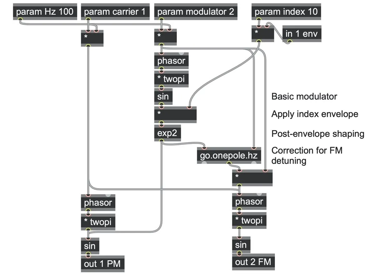
FMPM-exponential.maxpat

Exponential shaping tends to lessen the characteristic “glassy” sound of PM/FM as the index changes and instead imparts a more fizzy texture.

Note that the exponential function will only ever return a positive output. That’s because the closer you get to zero, the flatter the curve gets, so you can never quite reach it. So, as the modulation index increases, the average value of the signal will get more positive. In the FM case, this would have caused the output to rise in pitch, but—as before—we suppressed detuning in the patch above by adding a highpass filter.

Using AM for asymmetric PM spectra

As we have seen, the spectrum of a sinusoidal PM patch is symmetric: with a sideband below the carrier for every sideband above the carrier. This can sometimes be problematic when the lower sidebands fold around zero, and in other terms, it is generally uncharacteristic of natural sounds. One way to break this symmetry is to use a modulator waveform that is not perfectly symmetrical. Another is to amplitude modulate the PM output with a waveform that is synchronized to the modulator.

In either case, it’s not easy to design a modulation waveform to produce a specific balance of sidebands. But here’s a really interesting exception: If we AM the output of the PM patch with a “raised cosine” window that is synchronized to the modulator frequency, it can completely remove all the sidebands below the carrier, leaving only sidebands above it A raised cosine window for phase running from 0.0 to 1.0 looks like this (first in math, then in code):

e n (cos (2π phase) - 1)

exp(n * (cos(twopi * phase)) - 1)

The parameter “n” defines the sharpness of the window: the higher N gets, the thinner the windows get. Here is the graph of a raised cosine as a function of phase (the X axis), with a parameter “n” of 4.

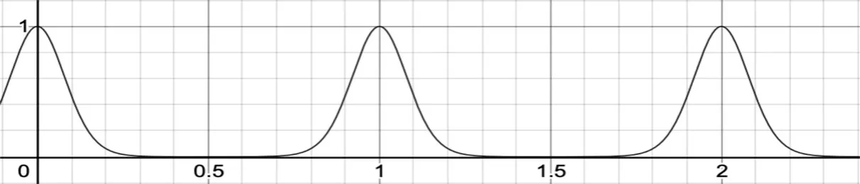
There is something particularly remarkable about this envelope function. If we drive it with the same phase as the modulator and set the parameter “n” to be exactly the same as the modulator index, and then we amplitude modulate the window with the phase modulation output, it perfectly cancels out all of the lower sidebands.

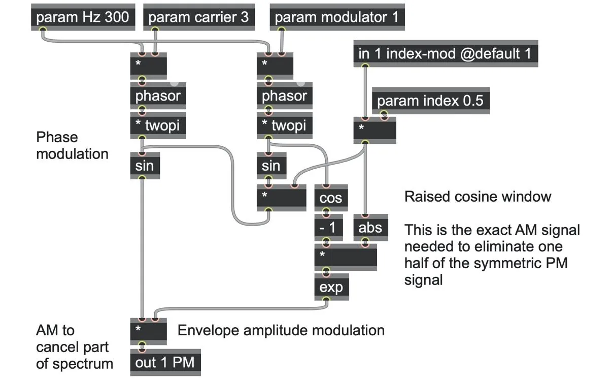
PM-asymmetric.maxpat

With a higher index, the resulting waveform begins to resemble an impulse train.

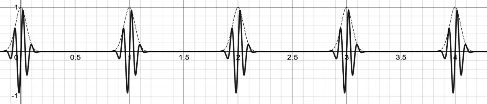
With a negative index, only the sidebands below the carrier pass through and all harmonics above the carrier are canceled out: a very alien sound.

Driving the in 1 index modulator with an LFO or oscillator can produce some quite rich sounds.

Things that can go wrong

We noted earlier in the Chapter that adding filters can be very helpful in suppressing clicks in phase modulation and suppressing detuning in frequency modulation, but here are a handful more recommendations for better control of your modulation patches.

Removing inaudible frequencies to preserve headroom

All of the techniques in this Chapter lead to the generation of new frequencies as sidebands. It’s quite possible that some of these sidebands appear in sub-audible ranges and even at zero Hz (DC); it is highly likely, for example, when carrier and modulator frequencies are very close to each other, which is especially the case for feedback modulation circuits! Any such sub-audible frequencies and DC offsets in the output will reduce the overall usable headroom of audio signals as they push it away from the zero-line. For this reason, you might want to place a dcblock operator or some other highpass filter tuned to around 10-40Hz after the carrier, just before the final output.

Aliasing and bandlimiting

We noted earlier in this Chapter that with AM/RM–and especially with PM/FM–using complex waveforms with significant high harmonics can very quickly produce sidebands at extremely high (and problematic) frequencies. But aliasing can be a problem even with pure sine waves. Although carrier and modulator signals cannot be above the Nyquist limit of samplerate/2, it’s quite possible for the sidebands generated to end up much higher. And since no sampled digital system can represent frequencies above the Nyquist limit, they will be “folded” back down (aliased), which can cause undesirably audible side effects. We’ll look at aliasing suppression in more detail in Chapter 9, but stated briefly here, the best way to avoid it is to constrain the input such that these frequencies are never generated in the first place.

In the case of AM and RM, it’s relatively easy. Since the upper sideband is C+M, then the maximum possible frequency of any AM or RM effect is the maximum absolute frequency of the carrier plus the maximum absolute frequency of the modulator. This suggests three possible solutions.

1. Pre-filter both carrier and modulator to have no frequencies above samplerate/4 so that their combination of samplerate/4 + samplerate/4 can never go above samplerate/2. (See AMRM-bandlimited.maxpat)

2. Oversample the AM/RM effect at 2x the normal samplerate, and downsample back afterward. (We will look at this kind of oversampling in Book 2.)

3. Or, if we have complete control over the waveforms, we can simply limit the total of the frequency parameters to never go above samplerate/2—such as by fading the inputs to zero when they approach the limit.

The first two options work with any waveforms and inputs; the third option requires that we know how to limit the inputs at the source.

The case of FM/PM is not as easy since far more sidebands are produced, and the mathematical Bessel functions that define the sideband intensities are quite complex. We can, however, point out a rule-of-thumb (known as the Carson bandwidth rule[88]) that pertains to the overall bandwidth when working with pure sine waves. This rule-of-thumb states that 99% of the signal energy in the spectrum is bounded between C - M*(index+1) and C + M*(index+1). With some additional refinements to handle negative parameters, the patching to implement this calculation looks like this:

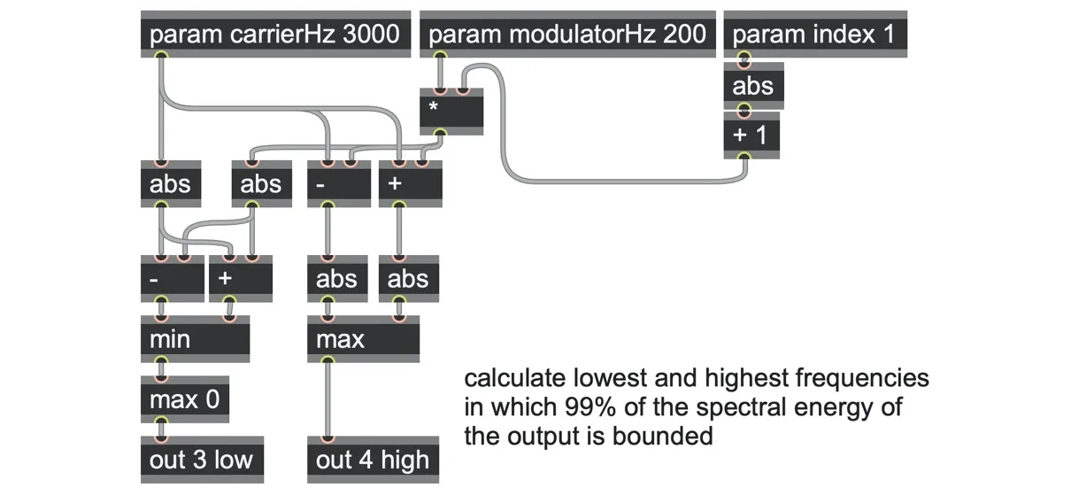
FMPM-carsonrule.maxpat

More usefully, we can rearrange this calculation to derive what the maximum possible modulation index can be within the Nyquist limit of samplerate/2.

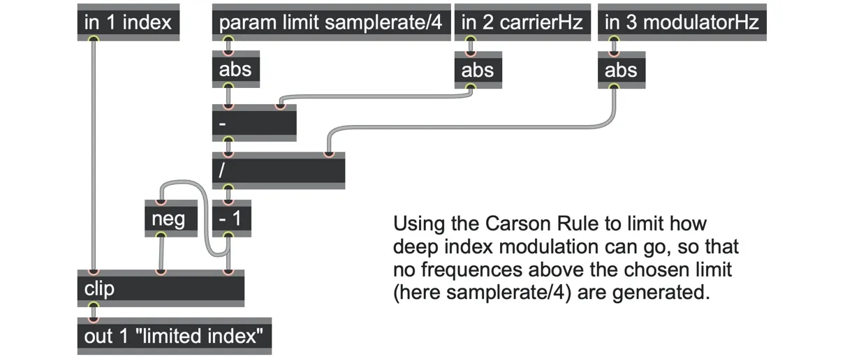
FMPM-carsonrule.maxpat

With these circuits in the FMPM-carsonrule.maxpat patch, you should be able to see how the param limit prevents the spectrum from going outside the defined upper bound, no matter what carrier and modulator frequencies you choose. For a slightly different approach, the FMPM-carsonrule-filtered.maxpat patch uses the rule to estimate a filter cutoff frequency to lowpass filter the modulation signal itself in such a way that it achieves a comparable limiting of the index; the result is a little less abrupt.

Remember, though: the Carson rule only works with pure sine waves. Different wave shapes, or more complex modulations, can easily introduce far higher sidebands. If these can’t be predicted and prevented at the source, a lowpass filter might be a better compromise.

The FMPM-antialias-filter.maxpat shows a simple example of inserting a two-pole lowpass filter, tuned to match the available bandwidth, which greatly suppresses high aliasing modulator frequencies even for a harsh saw wave modulator.

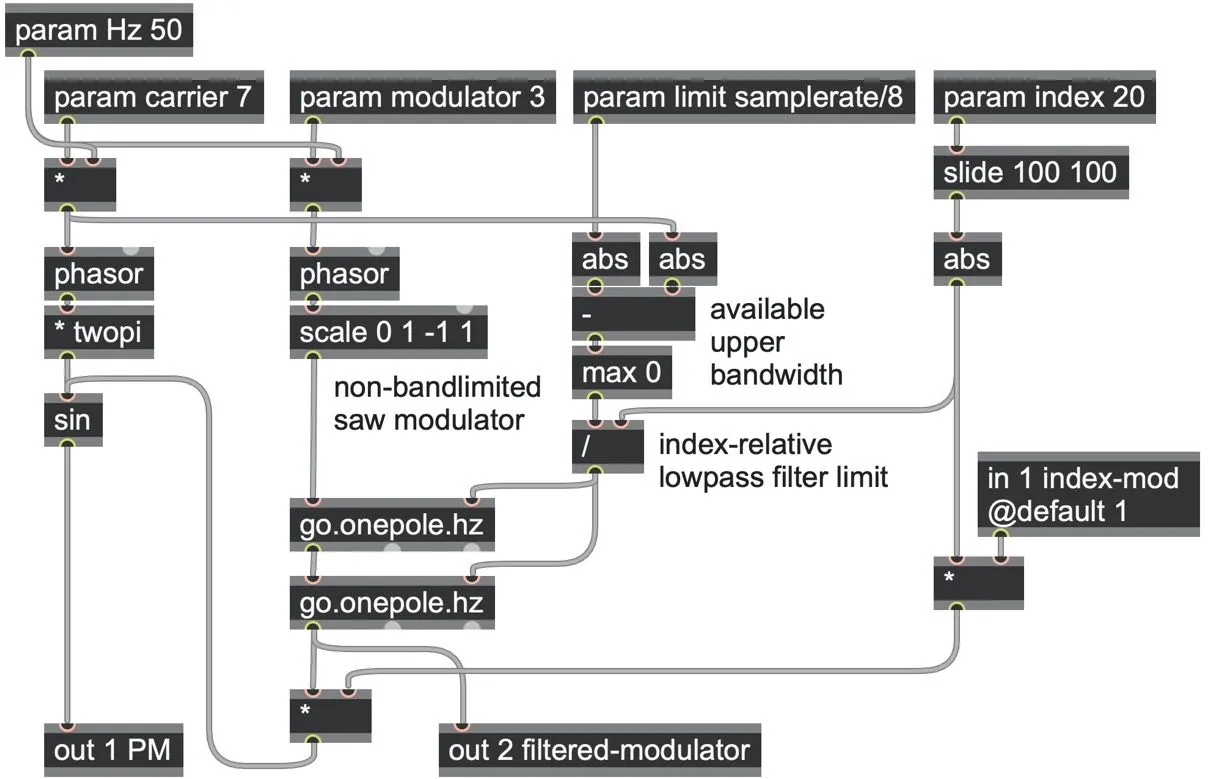
FMPM-antialias-filter.maxpat

Delay as phase modulation

In Chapter 7, we talked about how modulating a delay operator’s delay time parameter can approximate the effects of Doppler shift: the rising and falling of frequencies when an object is moving toward you or away from you. Now you might be able to see how this is the same as phase modulation. Modulating the delay time alternately compresses or expands the data read out of it, just as a moving object can compress or expand physical wavefronts emanating from it, thus raising or lowering perceived frequencies. This compression and expansion of the waveforms is like the effect of adding a continuous modulator to the phase input of an oscillator: according to the modulator, sometimes we are reading ahead, sometimes reading behind. Put another way: if frequency modulation is like a singer with extreme vibrato, then phase modulation is rather like a singer with no vibrato, but who is moving very quickly toward you and away from you

Since phase modulation is similar to a high-frequency Doppler shift, it makes sense that you can also use a variable delay to create phase modulation. We can certainly do this, but there are a couple of subtleties to work through first.

• Since the modulator signal normally represents a phase in radians, we need to convert that to an equivalent delay time in samples, which we can do by multiplying the modulator with samplerate/twopi.

• We might also want to scale this to the length of the carrier’s period so that a phase rotation of pi radians will phase shift by half a cycle, which we can do by dividing by the carrier frequency.

• Since a delay can only read from the past, not the future, there’s no such thing as a negative delay time. That means we can’t handle negative phase modulation. Instead, we must raise our modulation signal to be always above zero by adding an appropriate constant offset—the simplest way being to stick a + 1 operator right after the modulator’s sin operator. And as an extra precaution (in case of a negative index or carrier parameter), we can insert an abs operator right before the delay operator’s delay time input.

It looks like the following patch when put together. On the left is a typical phase modulation patch that we have seen throughout this Chapter. On the right is a patch that produces the same sound by feeding the modulator signal to set the delay time of a delay operator.

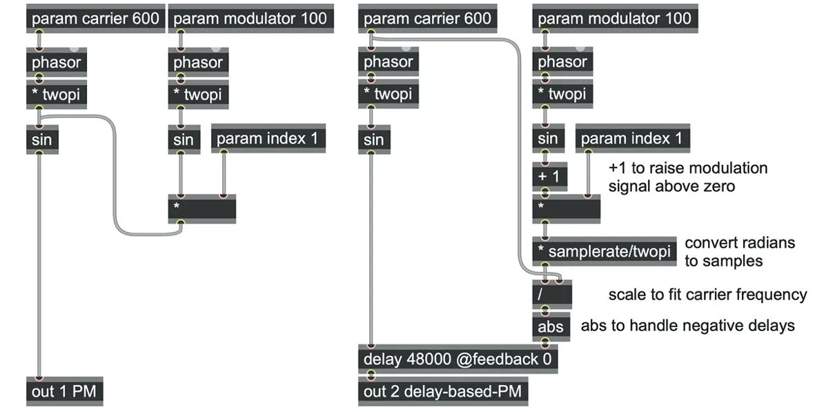
PM-is-doppler-delay.maxpat

Using a delay operator to implement phase modulation is more computationally expensive, but it does offer a unique advantage: it allows you to modulate any carrier signal, even one that you have no control over, such as a live audio input. However, it does then require that you either estimate the carrier frequency or else ignore this component of the delay time calculation and embrace phase modulation with a more arbitrary depth control.

More generally, we can use this insight to look again at delay-based circuits, knowing that we can introduce the various effects and transformations of PM through audio-rate modulation of delay time. For example, with a Karplus-Strong delay-based string model, dropping in a slight amount of delay-time modulation at one-half the string frequency can add some deliciously chorus-like subharmonic fuzz to the sound.[90]

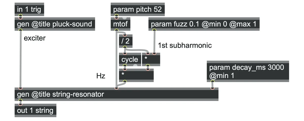
KP-FM.maxpat

However, for a more robust phase-modulated string model, the sinc-interpolated example at the end of Chapter 7 is recommended. We also noted in that chapter how modulating the cutoff frequency of a history or delay-based filter at audio rates can produce interesting timbral complexity; you might now understand this a little better through the lens of frequency and phase modulation!

Blending harmonic oscillators

The clangorous timbres that enharmonic ratios produce can be absolutely wonderful noises, but sometimes we might want to focus only on purely harmonic timbres. In that case, it’s tempting to restrict carrier and modulator frequencies to be simple whole number multiples of the fundamental frequency (where the “harmonicity” ratio forms simple fractions). It’s easy enough to limit a parameter to whole numbers via a floor operator, but then we wouldn’t be able to transition smoothly from one timbre to the next. As the parameter is changed, we would hear undesirable “stepping” in the output.

To solve this, and achieve smooth morphing between integer parameters, we can use a trick we have used several times in this book, such as the smooth bitcrusher in Chapter 5 and the mipmap level mixer we’ll explore in Chapter 9. The trick is to simply use two copies of an algorithm, each using a different parameter value, and smoothly crossfade between them to emulate one morphing parameter. To transition between two neighboring integer parameters, we can use two copies of the algorithm and a trio of floor, + 1, and a mix driven by the fractional difference to crossfade between them.

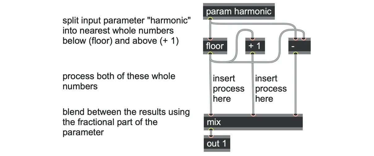
Now we can simply put our sine wave oscillators inside this structure to synthesize the two nearest harmonics. We can even save a little CPU (and gain a little stability) by having both oscillators driven by the same phasor input.

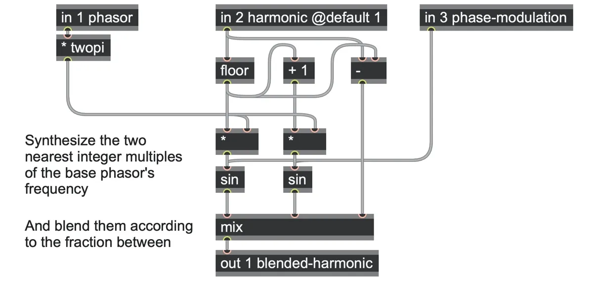
Harmonic.maxpat (and go.harmonic.gendsp)

This works because the multipliers coming out of the floor and + 1 operators are always whole numbers, and since sin repeats seamlessly every twopi radians, a whole number multiple of that also repeats seamlessly at the same point.

A fundamental phasor ramp at 1Hz (dotted line) and its harmonics at exactly 1x, 5x, and 6x this frequency (solid lines). Notice how all harmonics complete a cycle at the same time as the fundamental phasor at x=1, x=2, etc.

With the Harmonic.maxpat patch, try modulating the “harmonic” parameter up and down smoothly between 1.0 and 10.0, with all the decimal numbers between. Instead of hearing stepping, you will hear smooth transitions, sounding a bit like a filter sweep through the harmonic series. (We come back to this with Modified FM later).

Blended harmonic AM/RM and PM

We can plug this “blended harmonic” oscillator (which we saved as go.harmonic.gendsp) back into our various modulation algorithm patches. We can do this for either of the carrier and/or modulator oscillators. In the following AM/RM patch, we did both, using the same phasor for each.

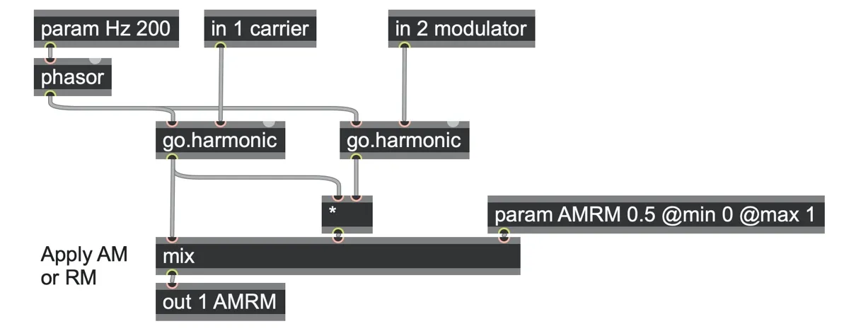
AMRM-blended-harmonics.maxpat

And we did the same for basic phase modulation.

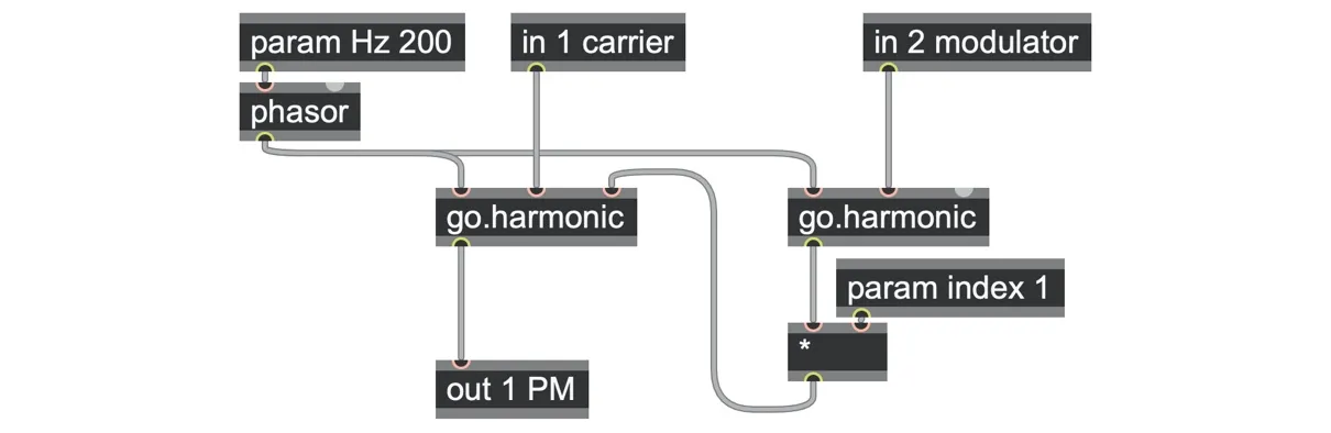
PM-blended-harmonics.maxpat

In both cases, the entire patch is now driven by a single phasor. The results have the characteristic complexities of AM/RM or PM and can be smoothly varied, but they avoid the enharmonic timbres because the frequencies are always whole number multiples of the fundamental phasor.

Try PM-blended-harmonics.maxpat with the carrier at 1.0 and the modulator around 1.15, and the index at 1.0, and you will get a soft saw-like waveform. Turning the modulator up to 2.0 produces a more square-like waveform. Turning up the index and modulator further produces sounds comparable to wavefolding. Adding some envelope, LFO, or oscillator modulation to the carrier and modulator inputs can lead to quite richly complex timbres while still maintaining a strong harmonic coherence. (If taking this modulation to extremes, it may be advisable to add a little lowpass filtering on them.)

Modified FM

The raised cosine window we saw in the asymmetric spectrum patch also does fascinating things with a blended harmonic oscillator. In this algorithm, called “Modified FM,”[91] a raised cosine window is driven by the same fundamental phasor that drives the blended harmonic oscillators, and both are combined by amplitude modulation.

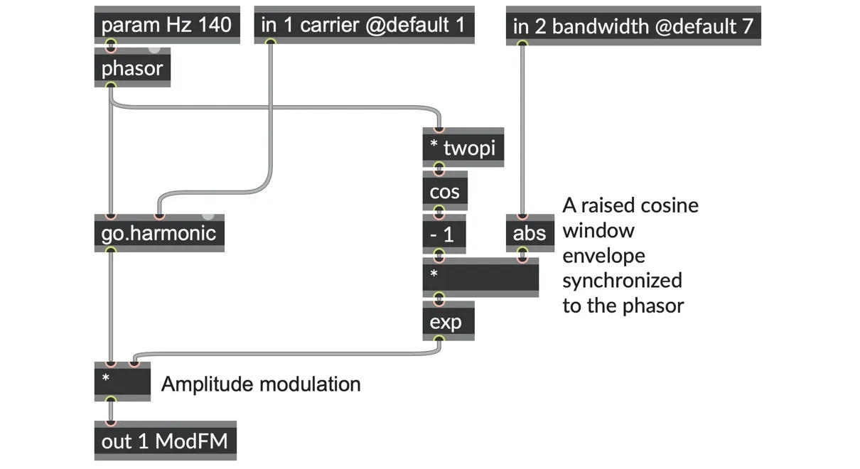
ModFM.maxpat

With this algorithm, turning up in 2 carrier operator shifts the center frequency up and down, much like a resonant filter, while modifying param index alternately narrows or widens the set of sidebands around this center frequency, much like a bandwidth or resonance control on a resonant filter. At certain settings, it can create a cheap band-limited approximation to an analog saw wave. At other settings, it can produce a characteristic acid-like impulse train, as below. The somewhat “vocal” formant quality has also led to its use for analysis-synthesis vocoding. We’ll look at some other ways of creating impulse trains in Chapter 10.