Chapter 6:
Filters, Diagrams, and the Balance of Time

You can use gen~ to implement many varieties of audio filters. While there are a lot of examples of audio filters that are specified using mathematical formulae, audio filters are also often depicted using "block diagrams" in textbooks and research literature. In this section, we'll look at how to use those block diagrams to guide your patching and recreate them using standard gen~ operators. We'll also use these to dig a little deeper into understanding what's really going on with digital filters in the time domain.

One-pole lowpass filter

Let’s start with a simple one-pole lowpass filter. Here is a typical block diagram for it:

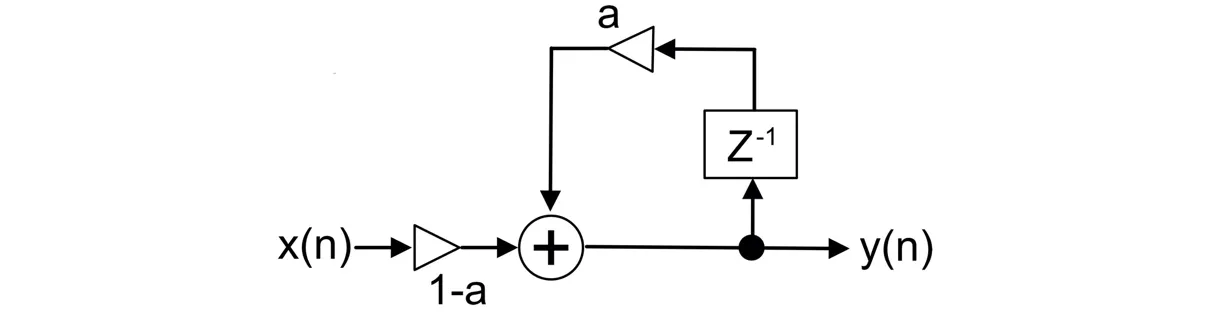
The block diagram is a kind of map of the flow of audio data through the filter from start to finish. The flow of data is from the left (starting at x(n)) to the right (ending with y(n)), with arrows also demonstrating the order in which calculations are done.

From blocks to operators

Implementing the filter from the block diagram is a matter of substituting the various graphic blocks with corresponding gen~ operators.

Here is what each one represents:

The "x(n)" represents the input signal sample value, which we can implement using the in operator.

The “y(n)” represents the output signal sample value, which we can implement using the out operator.

A circle with a plus sign (+) in it represents a point at which signals are summed together. Sometimes this is written with the Greek letter Sigma (∑), but it means the same thing. In gen~, we can implement this with an add (+) operator or simply by routing two or more signals into any operator’s inlet.

A Z-1 box is a convention used to represent single sample values. If Z0 represents the signal’s current sample value, then Z-1 is the previous sample value. In gen~, we can implement the “signal’s previous sample” Z-1 operation using a history operator. (If the diagram uses Z-N, this simply means the signal’s value N sample frames ago, Ih is a delay effect, and we can implement this using a delay operator.)

A triangle object represents an operation to multiply (amplify or attenuate) the input. It could be labeled with a numeric value, or the name of a parameter, or perhaps some mathematical expression of parameters. The block diagram at the start of this chapter contains two of them; one has a multiplier of "a," and the other has a multiplier of "1-a". In gen~, the operation of amplification/attenuation is a simple multiply (*) operator. The parameter can be replaced by a signal to its right inlet, for example, routed from a param object.

Turning Heads

Now we know what operators we'll use to patch our filter, how are they hooked together? In a 2014 SEAMUS workshop on physical modeling using gen~, Jon Christopher Nelson introduced a simple and elegant way to help translate a filter diagram to a gen~ patch, simply by rotating the block diagram 90 degrees clockwise. That simple transformation re-orients the diagram so that the information flows from top to bottom in a way that more closely resembles the flow of gen~ patching, making it more obvious how to wire them up. We'll do the same.

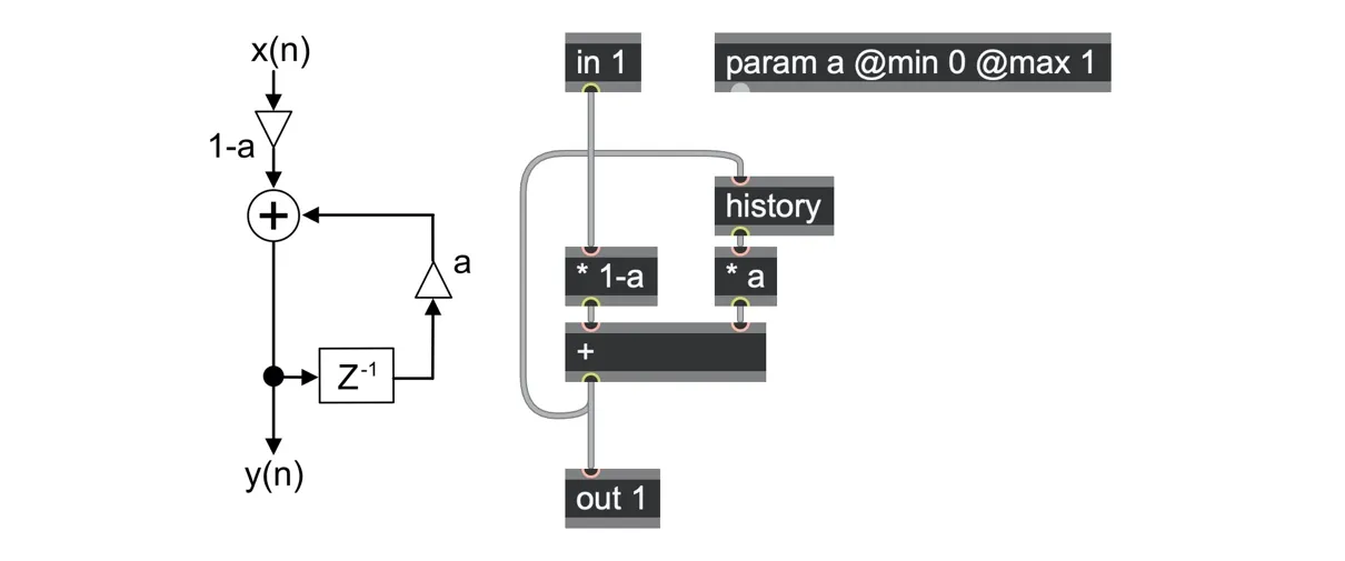
Note that since the two multiply operators refer to the same "a" parameter, we just added one param a operator and then used its name in both of the multiply operators.

The one pole low pass filter is one of the simplest filters you can build, and we'll see in the next section how we can patch it even more simply, however we'll also see how it hides within it several fascinating implications. But first, what is it useful for?

You can use it to smooth out control parameters, add slide and glide to pitch changes, and so on, and it also works as a simple audio filter, though it is not particularly exciting: it has a very gentle -6db/octave slope — the gain drops by half (-6db) as the frequency is doubled (one octave higher). If you want a steeper slope, you could chain a few of these one pole filters in series (each processing the output of the last), but—as we shall see later in this chapter—other filter architectures can be more effective for this. The humble one-pole filter does have a particular advantage, however: it will never overshoot the target or wobble (it does not "ring").

When is a filter more than a filter?

Before we go further, we'd like to point out several intriguing ideas lurking in this simple patch. We're mentioning this here because we think it's useful to develop the habit of seeing how circuits can be understood in more than one way. In this case, our one-pole filter can also be understood as an integrator, an averager, and a translator; you'll see all three of these perspectives used throughout this book.

Integration: Let's start by considering this patch as an integrator — that is, something that adds up everything it receives. You can see this in the feedback path that goes from the output through the history operator and adds back to the input — it's similar to the integration that an accum operator does, as we saw in Chapter 2. The difference here is that this integrator is "leaky": the multiplier of "a" (which is less than one) means that each time the signal goes through the feedback loop, a little bit of its energy is lost (and the multiplier of "1-a", which is also less than one, means that a little bit of energy from the new input is also lost). That's why this is called a "leaky integrator." The smaller the value of "a" is, the more the integrator leaks.

Averaging: How does this patch represent averaging? The key lies in asking what you get when you average two signals, X and Y. You get a mix or crossfade that is halfway in between them. Normally we think of the average as (X + Y)/2, but there are a couple of other ways of expressing that expression:

X + 0.5*(Y - X)	(0.5*X) + (0.5*Y)

Each of these three expressions works because both X and Y are given an equal weight of 0.5 each, and since 0.5 + 0.5 = 1.0, the total remains balanced. But these weights don't necessarily have to be the same. A "weighted average" changes the weight values, but it keeps them balanced so that the sum of both weights is still equal to 1.0. For example, if we used 0.8*X + 0.2*Y, we have an average that is balanced (since 0.8 + 0.2 = 1.0) but weighted more toward X than toward Y. For a more general weighted average, we can express it in terms of a common factor, a. Here are two equivalent ways to write this mathematically:

X + a*(Y - X)	(1-a)*X + (a)*Y
(as a line equation)	(as a weighted average)

The format on the left shows how this is a linear expression. if you imagine a straight line traveling from X to Y, then the “a” tells you how far you have traveled along that line. So, what this expression does is also called linear interpolation.

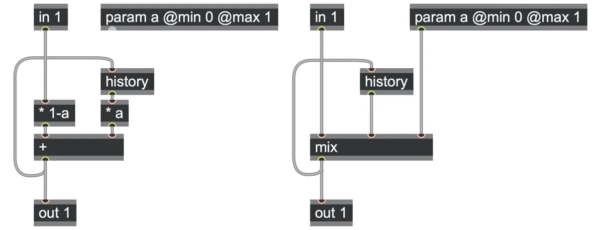
The format on the right is like a crossfader, where the variable a sets the crossfade amount. As we have seen earlier in the book, you can do this using the mix operator, whose inputs correspond to the values of X, Y, and a respectively.[50]

If you look at our one-pole filter patch again, you might notice that, at its heart, it has precisely the same weighted average expression as the mix operator, (1-a)*X + (a)*Y.

So, we can simply drop a mix operator in as a replacement, and the results of these patches will be exactly the same:

go.onepole.basic.gendsp

Seen in this way, what a one-pole lowpass filter is really doing is taking a weighted average between a signal and its own history, or equivalently, tracing a straight line from its history to its input!

Translation: Our final observation is that this circuit is also a translator. This is perhaps the least obvious aspect of the patch, but we can demonstrate it a little more clearly by rearranging our patch. Again, both versions are exactly equivalent:

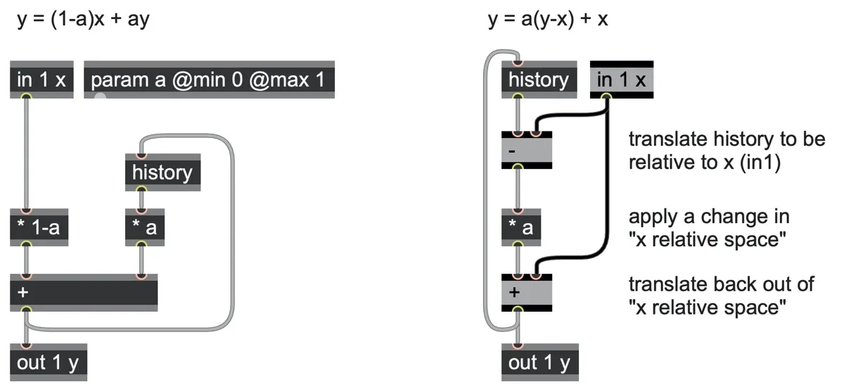
With the re-arranged version on the right, we can see that the recirculating feedback from the history operator is first translated to be relative to the input (by subtracting the in 1), then transformed in this relative state (by multiplication with param a), and then "un-translated" back to a non-relativized state (by adding the in 1 back again).

This technique of translating (or "projecting") a problem into a new space, applying a change more easily in this space, and then reversing the translation to return to the original space is a very general design pattern for solving problems, and we use it often in this book.[51] It is analogous to shifting a problem to a temporarily more convenient perspective; in the case of the one-pole filter above, we shift into a perspective that is relative to the input in order to make our history operator's feedback loop gradually minimize its difference from the input, and thus trend smoothly toward it. From this point of view, the signal at the history operator "wants" to get as close as it can to the signal at in 1 but can only do so sluggishly.

Setting the frequency

Let's feed our one-pole filter with a slow pulse wave to see how it responds. The balance parameter needs to be just slightly less than 1.0 for the effect to be visible.

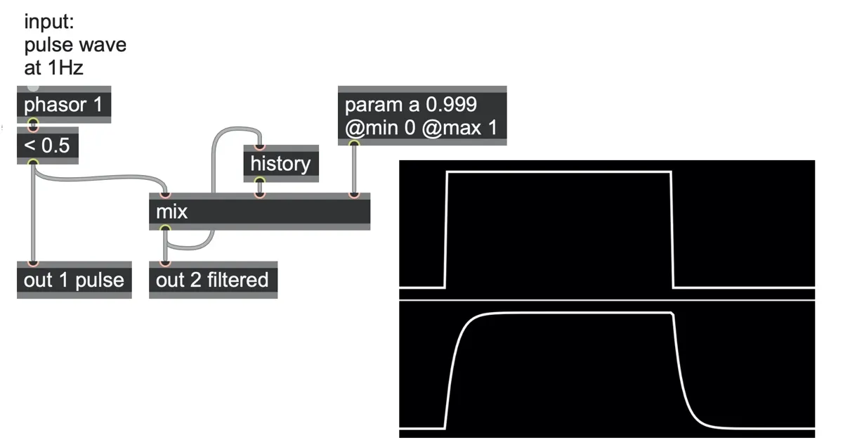
The top scope trace shows the original pulse wave, and the bottom scope trace shows the result of the mix operator with its own history.

So, over time, it smoothes the sharp edges, exponentially getting closer to the input signal. The filter coefficient (the 3rd input to the mix operator) determines how slowly or quickly it can do so. It's a kind of adaptive average of a signal, which tries to ignore any skittish divergences of the input and instead lazily focuses on following the signal's central trends. That's why we often use this kind of patch to smooth out noisy controls, such as removing clicks from sudden parameter changes and so on.

You might notice that the param a operator's setting is very sensitive: most of the interesting response is when the value is very close to 1.0. As it approaches 1.0, the curvature gets smoother and longer, and the sound output gets duller and darker. If param a is exactly 1.0, then we make no changes to our history, and the output holds constant forever. If param a is slightly below 1.0, then changes in the input will have only a tiny influence to pull the history this way and that; and only sustained changes (low frequencies) in the input will be able to significantly influence the history and the output. That is, in a lowpass filter the output is always trying to reach the input, and the param determines how slowly or quickly it can do so.

Thus param a determines what frequencies are slow enough to be followed by the history and thus pass through the filter mostly unchanged, versus what frequencies are too fast to be followed and thus lose power when passed through the filter. Typically, we express the balance point between these two regimes as the "cutoff frequency", which usually means the frequency which would lose half of its power (a loss of -3dB) when sent through the filter.

If you want to compute what the mix balance should be for a specific frequency cutoff frequency in Hz, you can use this calculation (first in math, then in code):

balance = e-2 PI |hz| / samplerate

balance = exp(-twopi * abs(hz)/samplerate)

Here is how this looks as a patch (left), along with the resulting spectrum when filtering a white noise source (right):

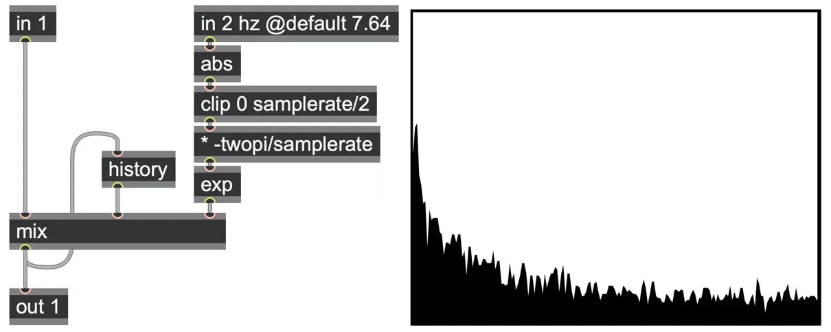
What's going on there? First, we take the absolute value of the cutoff value using the abs operator because negative frequencies should behave the same as positive frequencies (and otherwise, the exp operator's output will blow up). Then we added a
clip 0 samplerate/2 operator to keep the frequency within a range that the filter can reproduce. Then we divide the frequency by the samplerate to get a normalized frequency (between 0.0 and 1.0), and multiply by twopi, to get a normalized frequency in radians per sample frame (between 0.0 and twopi). That is, if this were a sinusoidal oscillator, this number is its angular rotation in radians per sample frame of real-time. Finally, this is made negative and passed through an exponential exp operator to balance the fact that a feedback loop will have an exponential decay: the longer the decay, the closer this exponent gets to 1.0.

Did you notice in that last example that we used an in operator rather than a param operator to set the frequency? While a param operator is a convenient way to explore a patch, it has a slight drawback when it comes to modulating a filter — changes to a param operator come from outside of gen~ and are updated at best only once per signal vector (i.e., the number of samples that Max or RNBO processes per object as its scheduler runs), rather than at the single sample rate that gen~ operators use. That difference may result in stepping, popping, or other filter glitching if you try to modulate it quickly. In most cases, filters behave better if their control parameters modulate smoothly. To be able to modulate with continuous audio rate signals, we replaced the param operator with an in 2 operator, which responds at full sample rate. (Alternatively, you could add a smoothing filter to the parameter itself. That will smoothen the parameter but will also limit how quickly our filter can be modulated.)

Half-lives: setting a filter decay in seconds

There's another way we can set the response of the one-pole filter that is particularly useful when using the filter to smooth out low-frequency modulations and parameter controls: by setting the "response time" in seconds.

The one-pole lowpass filter has an exponential response: given a step input, it will output a curve that gets flatter and flatter as it approaches the target. This is called an exponential decay. These are reminiscent of many natural phenomena, including the typical responses of physical instruments. This stems from the unique nature of the mathematical function y=ex (represented in gen~ by the exp operator), defined as the function whose slope (i.e., its rate of change) is equal to y. That is, the slope of ex is equal to the output of ex. For example:

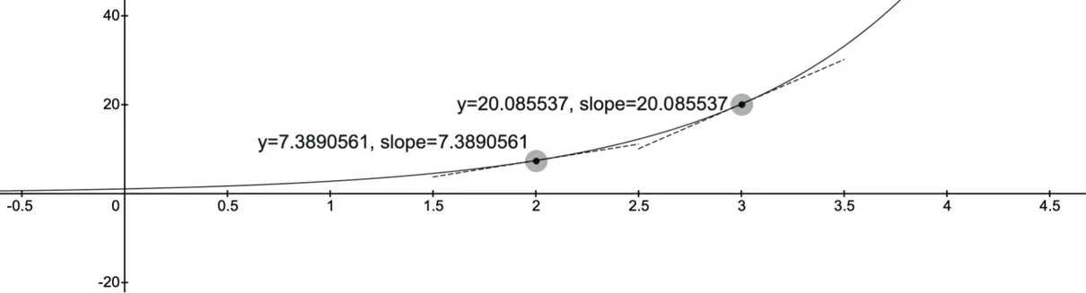
Any function whose growth rate is proportional to its size, as seen in population growth, compounded interest, etc., can be written as an exponential function of time multiplied by a growth constant. The growth constant identifies how sharply the exponential curve rises.

The same holds for systems showing exponential decay, except that the growth constant there is negative and identifies how sharply it falls. Here, for example, is e-x:

This sharpness of exponential decay is a kind of "characteristic time". Radioactive elements have a characteristic half-life, which is the amount of time by which 50% of a clump of that element will probably have decayed. Similarly, in audio, we can talk about the characteristic decay time of a reverberator, delay, or other resonator. A widely used measure for this is the T60 time, which is the time for an input signal to decay by -60db. Since every -6db halves the amplitude, -60db simply means a fall in amplitude of 2-10, which is very nearly 0.001. Why this level? Because it is a convenient number that is close to a threshold of auditory perception.[52]

If you play a calculator game, starting with a value of 1.0, how many times can you multiply it by 0.5 until you get below 0.001? How many times if you multiply by 0.9? How many times if you multiply by 0.999? These decay multipliers (0.5, 0.9, 0.999) each specify a different T60 time in terms of the number of multiplications needed to reach 0.001. If we apply this multiplication once per sample frame (as we do in the one-pole filter), the number of multiplications equals the T60 time in sample frames.

In gen~, the t60time operator will tell you exactly how many of these multiplications (how many sample frames) a given decay multiplier will need to decay by -60db. The t60 operator does the opposite: it will tell you what multiplier you need to decay by -60db over a given number of multiplications.[53] With this, we can create very natural decays with precisely specified durations.

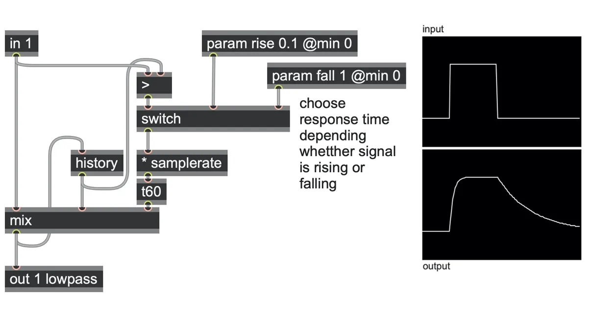
And, it turns out, we can feed this directly into our mix & history one-pole filter.

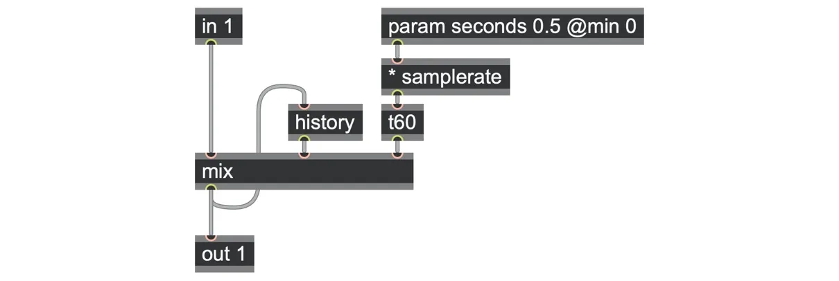
The one pole filter's exponential response can also create quite natural sounding envelopes. You might want to use different response times for rise and fall, depending on whether the envelope is rising or falling.

A lowpass gate (LPG)

Let's build on that last example to create a lowpass gate (LPG).[54] A lowpass gate is a particular kind of analog synthesizer circuit originating with the Buchla 200 modular synthesizer series that came to be highly regarded (and remains popular today) for its natural enveloping qualities.

Here, the envelope is not simply applied by amplifying and attenuating an audio input signal, but by opening and closing a lowpass filter according to a control signal:

• When the control signal is zero, the cutoff frequency of the filter is well below the audible frequency range, so no audio passes through the filter.

• As the control signal is increased above zero, the cutoff frequency rises into the audible range so that more of the audio at the input now passes through the filter.

Additionally, the Buchla design used a vactrol[55] to process the control signal input, which adds a characteristically gradual response: even using a sharp-edged logic gate signal to drive the lowpass gate will result in a smooth opening and a more gentle closing of the filter envelope. That smooth and nonlinear behavior makes a lowpass gate a good source for imitating the timbral changes of natural percussion sounds.

Our lowpass gate patch thus requires two basic components — the lowpass filter itself and some patching to emulate the behavior of a vactrol. Let's start with the vactrol emulation.

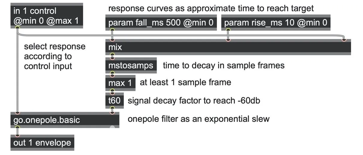
go.vactrol.gendsp

Two param operators set the response times in milliseconds for the extremes of the control input. The control value from the in 1 operator is used with a mix operator to blend between these two response times; when the control is 1.0, we use the param rise_ms time, and when the control is 0.0, we use the param fall_ms time. For any intermediate control value, we use an intermediate response time. This is then converted to samples using an mstosamps operator and then processed through the t60 operator we've just examined to set the signal decay coefficient (the time to reach -60dB) for a go.onepole.basic abstraction, whose job is to smoothen out the control signal for the vactrol output.

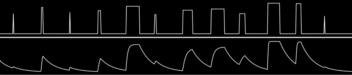
Here is the result of feeding some randomized gates (top scope) into the go.vactrol abstraction and the emulated vactrol's output (bottom scope):

We can then use this vactrol output as an envelope to open and close a lowpass filter to complete the lowpass gate. For example, in the following patch, we use it to drive three onepole filters arranged in series so that the rather gentle -6db slope of a one-pole filter becomes a steeper -18db slope. We also used a scale operator to map the envelope shape to a more expressive frequency range.

The scope in the following image shows the effect of this lowpass gate on a square wave oscillator:

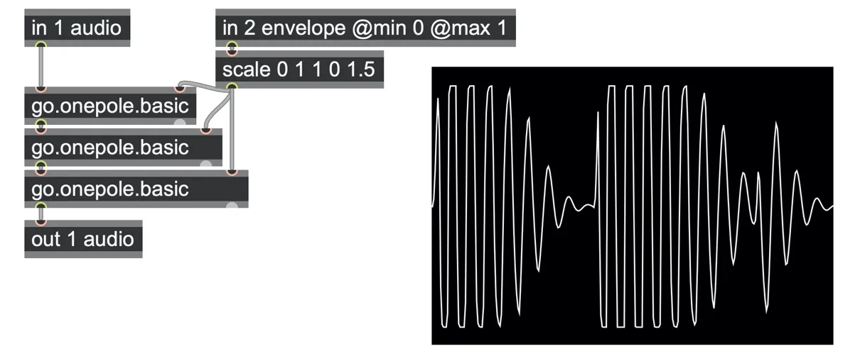
lowpass-gate.maxpat

There's no need to limit yourself to a simple lowpass gate emulation like this, of course. For a more interesting filter-based envelope, we can use a more interesting filter and more configurable control over the envelope response.

In the following patch, we used both lowpass and peak bandpass outputs of the go.svf trapezoidal state variable filter (which we will build later in this chapter) and added some additional parameters to control its response. (The go.equalpower abstraction is included to perform an energetically balanced mix between the two filtered signals, resulting in a more exaggerated response.)

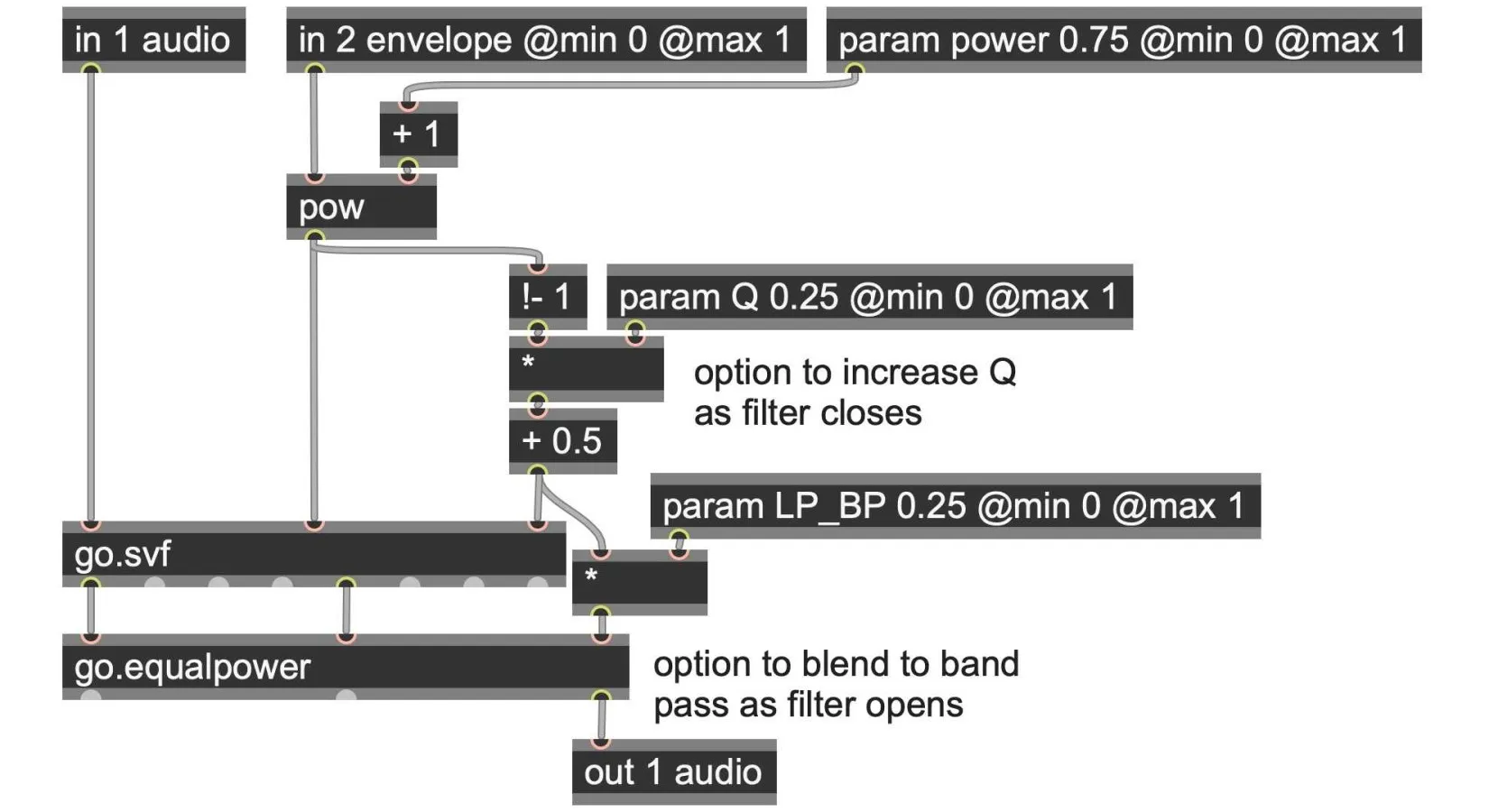
low-pass-gate.maxpat

A lowpass gives you a free highpass

Here is another trick: subtract the one pole's output from the original signal, and you get a complimentary highpass filter. If you think about it, by taking away a smoothed version from an input signal, the residual you are left with is all of the "non-smooth" differences; that is, the deviations away from its average.

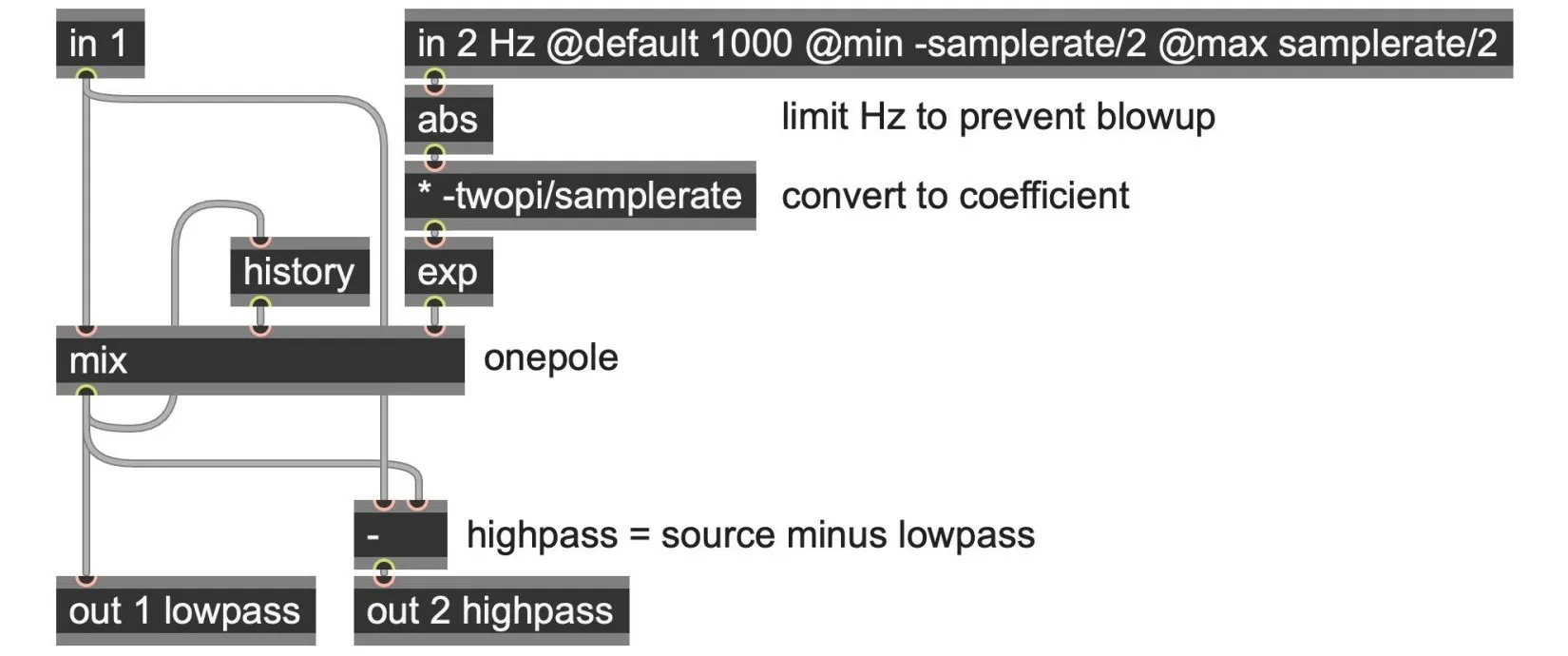
go.onepole.basic.hz.gendsp

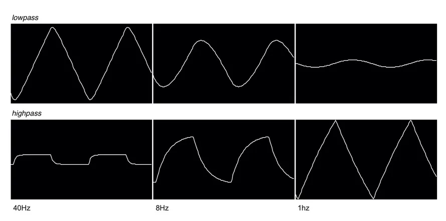
The images above show the effects of filtering an 8Hz triangle wave with the cutoff frequency at 40Hz (left), 8Hz (center), and 1Hz (right). The lowpass filter (top row) softens the signal, rounding its corners, while the highpass filter (bottom row) captures what was lost in that lowpass. Notice how in the 40Hz case (left), the highpass seems to represent the slopes of the original signal more than the signal itself. In the 8Hz case (center), both filtered signals are closer to representing the original waveform but notice how they are also shifted in time relative to the original signal.

In the 1Hz case (right), now the highpass most closely represents the original, with the lowpass capturing what was taken away. It makes sense: changing the filter frequency is changing the mix parameter, and that is changing the balance between the original signal and its changes in a history operator. (As we noted earlier, a lowpass filter approximates an integrator, and now we can see the highpass approximates a differentiator, where the filter coefficient sets up the balance between a signal and its changes.)[56]

A common use of this one-pole highpass filter is to recenter a signal around the zero line. Imagine you have a signal that has a continuous value of 0.5. The running average (lowpass filtered version) of this signal is, of course, 0.5, while the deviations from the average (highpass filtered version) of this signal are zero.

Whatever the input, a lowpass will try to recenter itself on the signal's average, whereas a highpass will try to recenter around zero. They will recenter gradually if the cutoff frequency is low or very quickly if the cutoff frequency is high. (This is also known as a DC blocking filter, where "DC" is short for "direct current," an analog electronics concept of any constant or extremely slowly changing offset that takes the signal average away from zero volts.)

It's especially important to apply DC-blocking highpass filtering in a feedback delay line or reverb algorithm. Otherwise, the delay can build up any low frequency or constant components until it saturates well beyond acceptable signal amplitudes! We'll see this again as we build physical models in Chapter 7 and frequency modulation in Chapter 8. This routine is so useful that there's a built-in operator specifically for this purpose: dcblock. The dcblock operator is a highpass filter below 3Hz.

Allpass filters

Our next block diagram example is an allpass filter. Allpass filters pass all frequencies evenly, which means that they don't shape the frequency spectrum of a sound at all: by itself, the output will sound essentially the same as the input. So how is an allpass filter useful?

What an allpass filter does is to delay different parts of the frequency spectrum by different amounts, which can create differences in phase. Normally, we can't directly hear phase changes, but we can when they are mixed with other versions of the original signal. For example, we'll see that if you mix the result of a chain of allpass filters back with the raw input, you get a classic whooshing "phaser" effect. Or, you can use an allpass filter to counteract unwanted phase shifts that another filter might have created. Or, if you mix several allpass-filtered signals together, you can create a sense of spaciousness as the signal phases are decorrelated from each other. For this reason, allpass filters are often found within reverb algorithms.

Let's start by noting something that you're likely to encounter as you start looking for filter block diagrams. You may discover that - just as there's more than one way to represent a mathematical equation or more than one way to represent an algorithm as a patch - there's also more than one way to represent a given filter as a block diagram. For example, you might find allpass filters described using any of the three following diagrams:

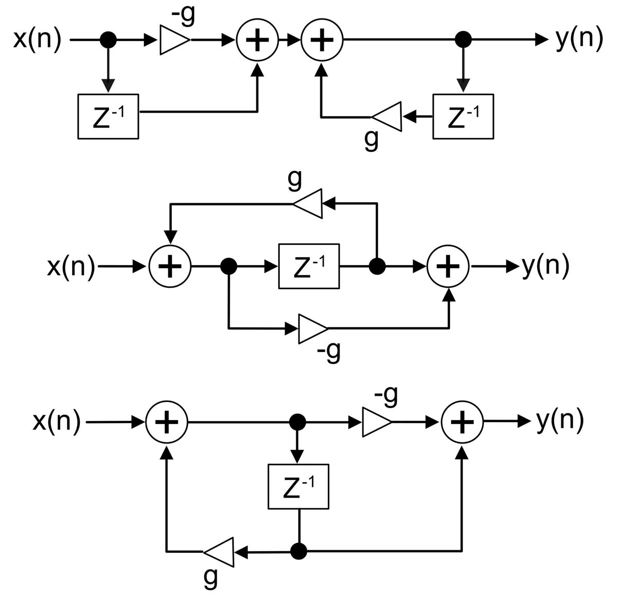
Although these three block diagrams look quite different on the surface, when you work through the underlying operations, you will find that remarkably they produce the same results. You could take any one of them as a starting point for translating into gen~. We're going to pick the one at the bottom, and as before, start by rotating the diagram 90 degrees clockwise so that the flow of data is top to bottom.

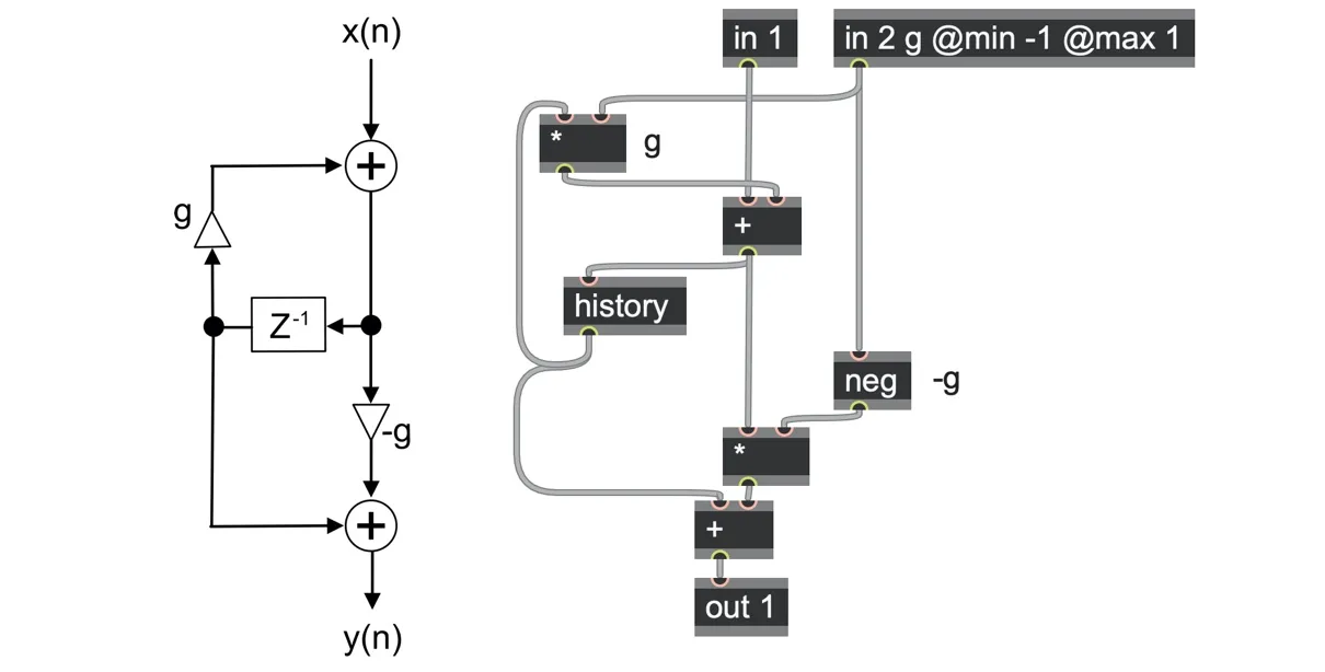
go.allpass.gendsp

After the rotation, we replace portions of our block diagram with the corresponding gen~ operators. We needed two * (multiply) operators — one for each of the feedback (g) and feedforward (-g) parameters, and two + (add) operators for summing. We added a single in operator for the g/-g values as well. Note that we also added @min -1 @max 1 arguments to our in 2 operator to constrain the range of the coefficient within safe limits.

Phaser

We can create a simple four-stage phaser effect by processing an input sound through a series of four allpass filters and mixing the result back with the original input.

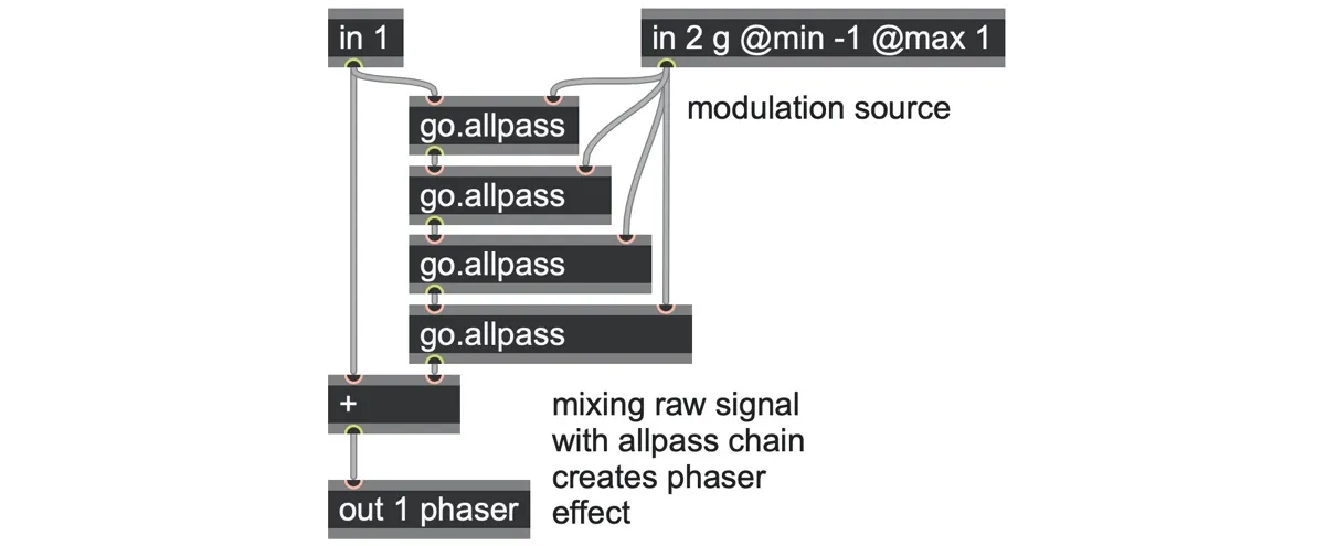
phaser-4stage.maxpat

On the next page we extended that patch to eight stages, with a selector to choose how many stages to use, and a feedback path to create a more resonant phasor.

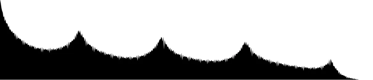
The resulting spectrum on a low frequency pulse wave, with the phaser-8stage-resonant.maxpat using all 8 stages set to a coefficient g=0.5 and feedback level fb=0.85.

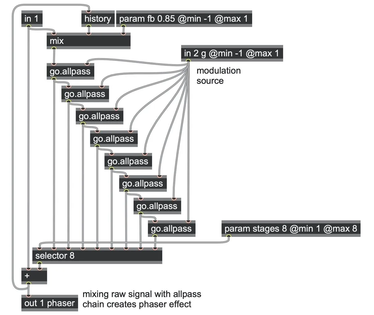
phaser-8stage-res.maxpat

Computing the allpass coefficient from a frequency

To compute the coefficient g from a desired frequency, we start by computing the angular radians per sample, which represents the rate of rotation of a sampled sinusoid at the desired frequency. We can compute this from a frequency in Hz using abs(frequency) * twopi/samplerate, the same conversion we saw with the one pole lowpass filter. From this angular radians per sample w we can derive the required coefficient g as (sin(w)-1)/cos(w).

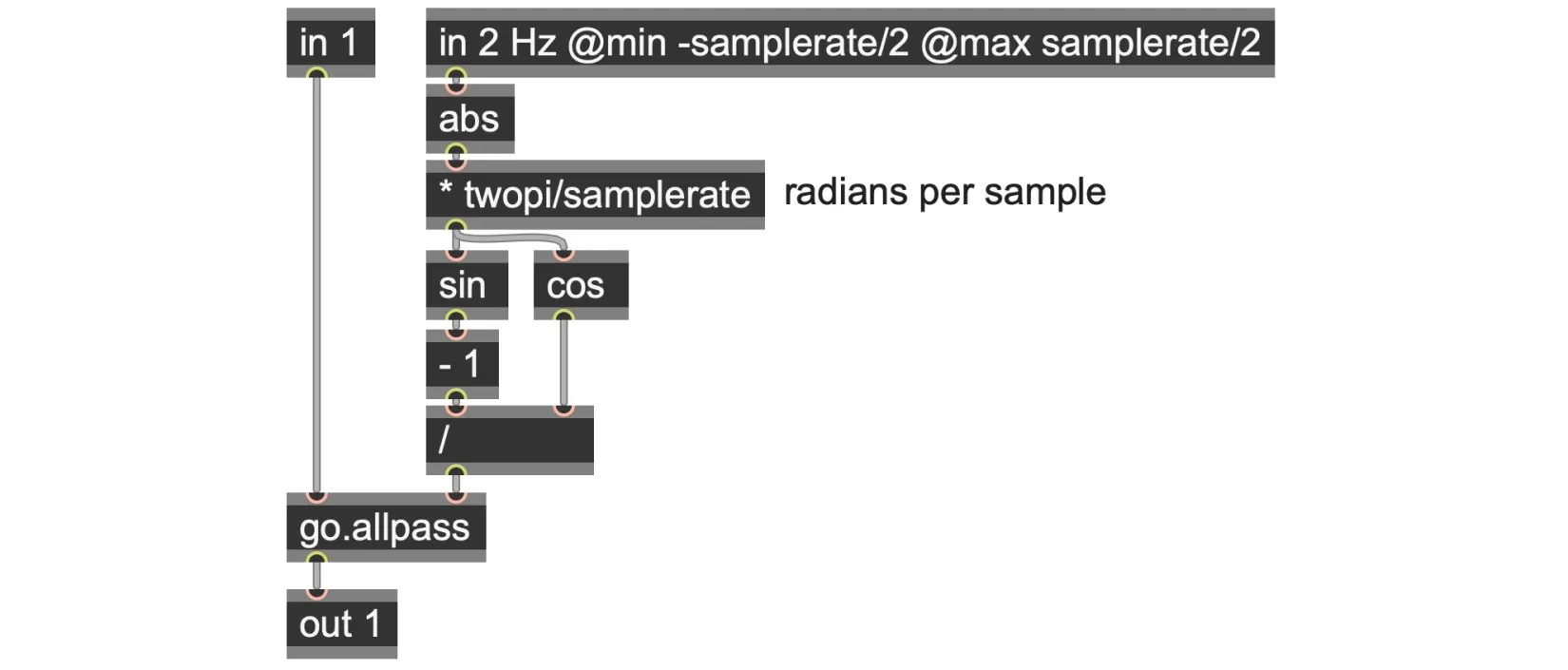
go.allpass.hz.gendsp

Biquad filters

Let's take an in-depth look at one of the most widely used digital audio filters: the biquadratic (or biquad) filter. This incredibly versatile general-purpose filter can be set up for many configurations–lowpass, highpass, bandpass, notch, highshelf, lowshelf, allpass, etc.–by doing nothing more than adjusting the parameters (also known as coefficients) of the filter. Here is a typical block diagram of a biquad filter:

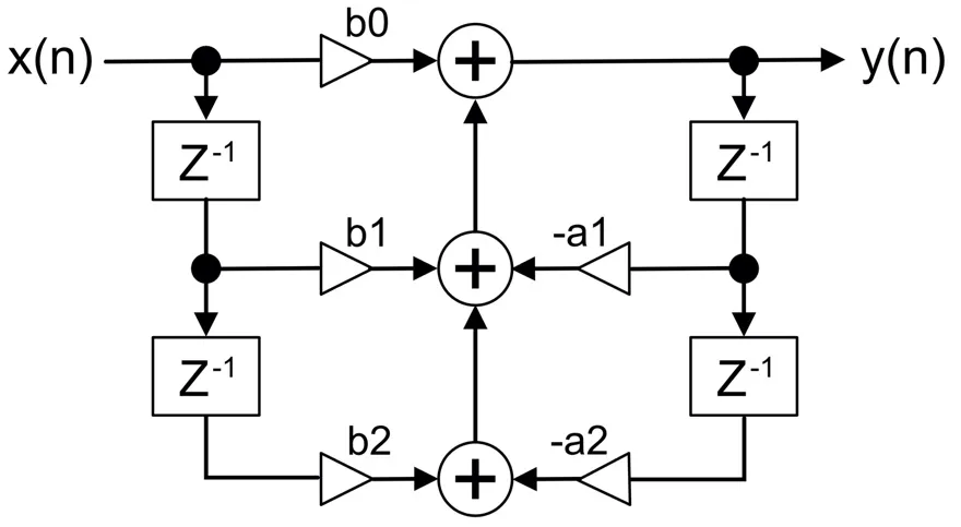
The biquad filter architecture has a direct path from input to output (via b0), as well as two feedforward sample delay paths (via b1 and b2) and two feedback sample delay paths (via a1 and a2), but otherwise doesn't introduce any new concepts. (You can compare this with the allpass filter in the previous section, which has one feedforward and one feedback path.)

As we've done before, we rotate the block diagram 90 degrees clockwise, drop in gen~ operator substitutes, and wire them up.

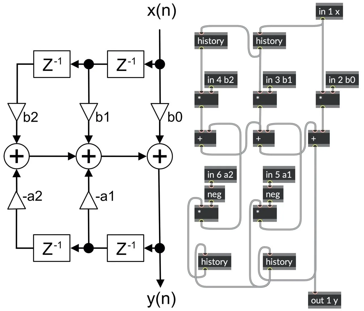
As a patch, this looks pretty tangled. We can clean it up by moving things around a little, and we can also make a few modifications to simplify the patch.

The a1 and a2 coefficients in the block diagram are labeled as negative values (-a1 and -a2). We can simplify this patch slightly by removing the neg operators and instead replacing + (plus) operators with a - (minus) operators. That's because subtracting the result of the multiplication with a coefficient is equivalent to adding a multiplication with the negative of that coefficient.

We can also simplify some of the patching, removing the need for + (plus) operators by connecting multiple patch cords to the next operator's inlet. This is because gen~ operator inlets always handle multiple incoming connections by summing multiple signals together.

The result looks a lot simpler:

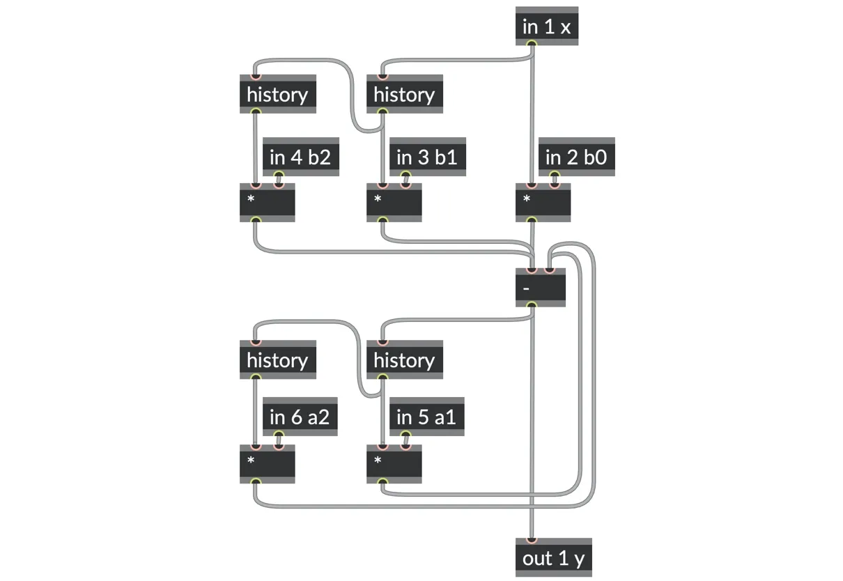
go.biquad.gendsp

Depending on how you're using the biquad, you might also want to add some limiting after the output to protect our ears and hardware; it could be one of the sigmoid bipolar waveshapers from Chapter 3 or simply a hard limiting clip -1 1 operator. This is because it is quite possible to set the input coefficients for the biquad filter in such a way that the filter feedback "blows up."

The one-pole filter we built earlier in this chapter took care of that by simply setting bounds for the filter coefficient, but due to the complexity of the biquad circuit, we cannot ensure this by clipping the coefficients, so instead we may need to limit the signals somewhere in our patch before it reaches our ears.

Biquad Filter Coefficients

Now we have a biquad filter; how do we use it? The digital signal processing literature has many examples of algorithms we can use to compute the coefficients for different filter types (lowpass, highpass, bandpass, etc.) and for different cutoff frequencies, resonance/Q, and gain factors.[57]

While a detailed description of how these values are derived is beyond the scope of this book, we can certainly implement them in gen~. In fact, we have done exactly that, with the go.biquad.lp (low pass), go.biquad.hp (high pass), go.biquad.bp (band pass), go.biquad.res (resonant band pass), go.biquad.np (notch pass), go.biquad.ap (all pass), go.biquad.ls (low shelf), and go.biquad.hs (high-shelf) abstractions, which you can drop into your patches as you need.

However, if you look closer at the equations of many of these common filter types, you might notice that many share a lot of the same underlying computations.[58] In fact, we can conveniently build a coefficient calculator for all of these filter types, optimized to make use of the many calculations they share:

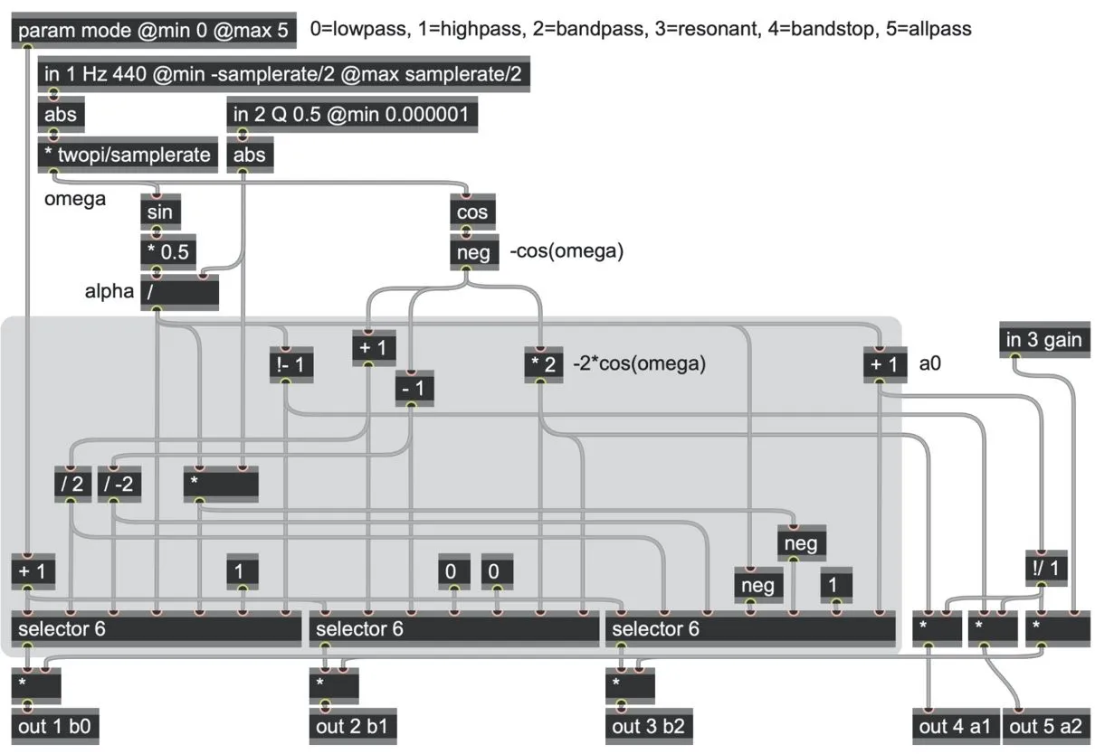
go.biquad.coeffs.gendsp and biquad-coefficients.maxpat

In this go.biquad.coeffs abstraction the highlighted part of the patch is the only part that differs between each filter type.[59] Using the selector operators here to route the different b0, b1, and b2 calculations is more efficient than switching between six completely different biquads. Looking for opportunities of shared computation like this is a good patching habit!

Cascades

Apart from the flexibility of creating many filter types just by changing coefficients, the biquad filter is also useful in how it can be cascaded in series to create more complex filters. Our humble one-pole filter achieved a 6dB per octave slope due to it having one feedback path. The biquad, with two feedback paths, achieves a steeper 12dB per octave falloff. So, if you wanted an even more "aggressive" filter with a steeper falloff, you might imagine adding more feedback paths. Unfortunately, such circuits can get increasingly susceptible to numerical instability and more easily blow up. Fortunately, we can achieve the same result through a "cascade" of biquad filters in series, all using the same coefficients.

The following block diagram arranges two biquads in series to achieve a 24dB per octave falloff.

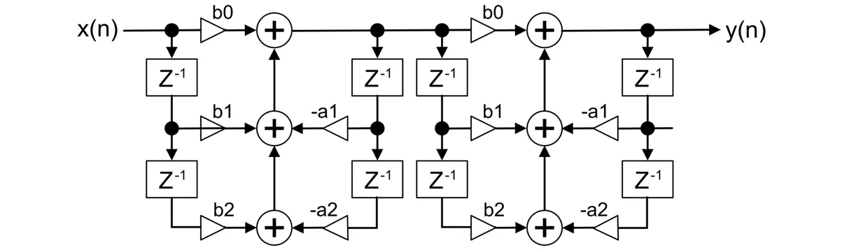
The next patch goes even further: four go.biquad abstractions are serially connected with a single go.biquad.coeffs abstraction converting filter cutoff, Q, and gain values to supply the same coefficients to all four abstractions. You can see the difference in filter roll-off in the visual displays. The fourth output, as a series of four biquads, has an extremely sharp falloff of 48dB per octave!

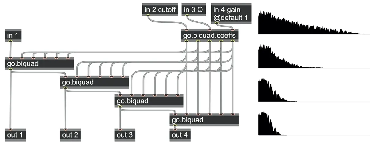
biquad-cascade.maxpat

The software with this book includes a go.biquad4 abstraction that chains four biquads in series (using the same coefficients), and there are also variants of each of the common filter such as go.biquad4.lp, go.biquad4.hp, and so on.

Another approach to cascaded filters involves configuring several biquad filters for different modes and controlling each filter individually. This can be particularly interesting when the filter parameters are modulated. The following example uses four biquads: one as a lowpass filter, two as resonant filters, and one as a highpass filter, each of which allows for the specification for the filter cutoff ranges individually.

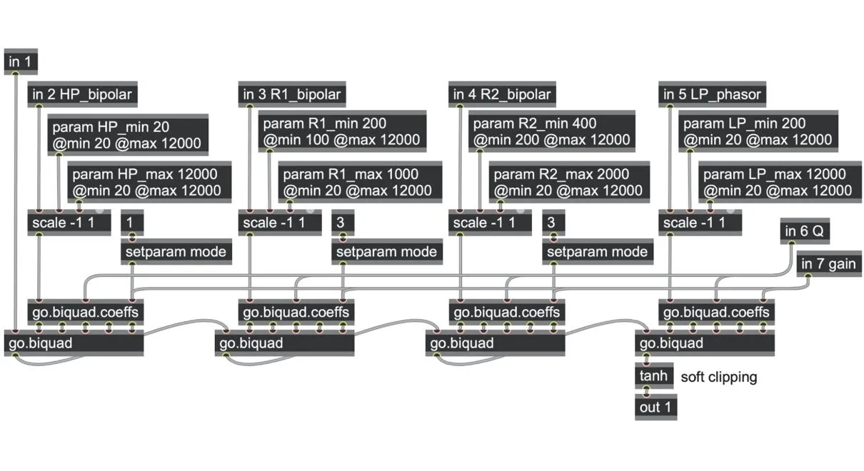We can then use LFOs running at different rates to modulate the filter cutoff frequencies of each of these filter sections continuously, and the morphing_biquad_cascade.maxpat patch lets you experiment with various filter ranges for each.

Trapezoidal filters

We saw earlier in this chapter that a one-pole lowpass filter is effectively a weighted average between the filter's input and its output. A more subtle point is that the timing is thus slightly skewed: it is a mixture of the current sample frame's input with the previous sample frame's output. This means that the phase response (the frequency-dependent delay) will also be skewed. Lower frequencies that are passed through the filter mostly unchanged will have almost no delay; higher frequencies that are attenuated by the filter are more significantly influenced by the previous output and thus have a greater delay. When combined with other filtering processes or when filtering under high-frequency modulations, these frequency-dependent delays and phase responses can make a real difference. But there's an alternative topology we can use, sometimes called the trapezoidal or bilinear transform, which can better balance this temporal skew.

To understand how this works, we can first look at integrators since we have already seen that integrators are at the heart of all filters. Here are two simple integrators:

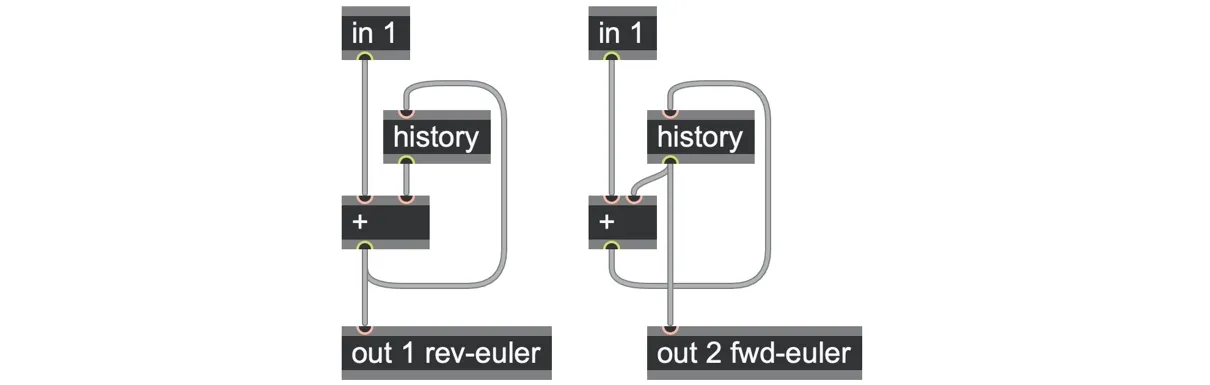
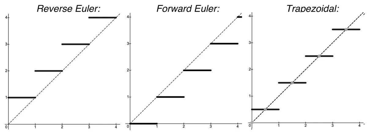
The one on the left is like the accum operator: it outputs the signal plus the integrator's previous value. It is also known as reverse Euler integration. With an input signal of 1.0, it will count from one with a series of 1.0, 2.0, 3.0, etc.

The one on the right taps the output at the history operator instead, so we get the current count plus the previous input; this is called forward Euler integration. This is effectively the same as the patch on the left but delayed by one sample, such that the new count appears on the next sample frame. With an input signal of 1.0, it will count from zero with a series of 0.0, 1.0, 2.0, etc.

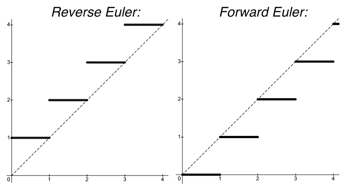
Where the circuit on the left is biased toward the signal at the end of a sample frame, the one on the right is biased toward the value at the start of a sample frame. But wouldn't it be better to avoid bias to either end and approximate the signal in the middle of the sample frame instead? This is what the trapezoidal architecture does, producing an average between forward and reverse integration. There are two ways to do this.

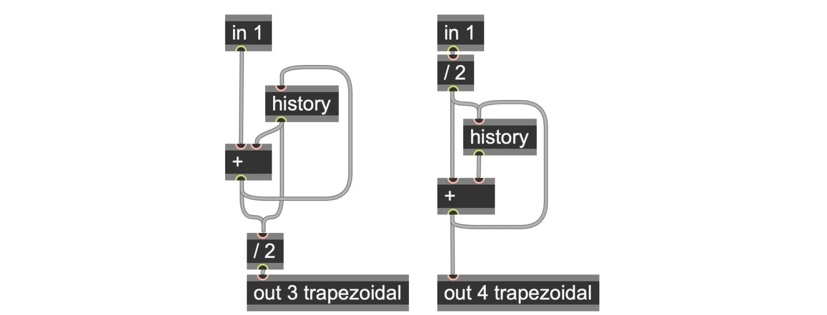
Look at the patch on the left: it takes both of the outputs that the reverse and forward integration used and averages them (using the / 2 operator). So, with an input signal of 1.0, the output will be 0.5, 1.5, 2.5, etc.–exactly the midpoint. (It is a counter with a delay of one-half of a sample frame.) On the right, we achieve exactly the same result simply by splitting the input into halves instead of averaging the output.

This is the format that the integrator is usually presented in block diagrams.

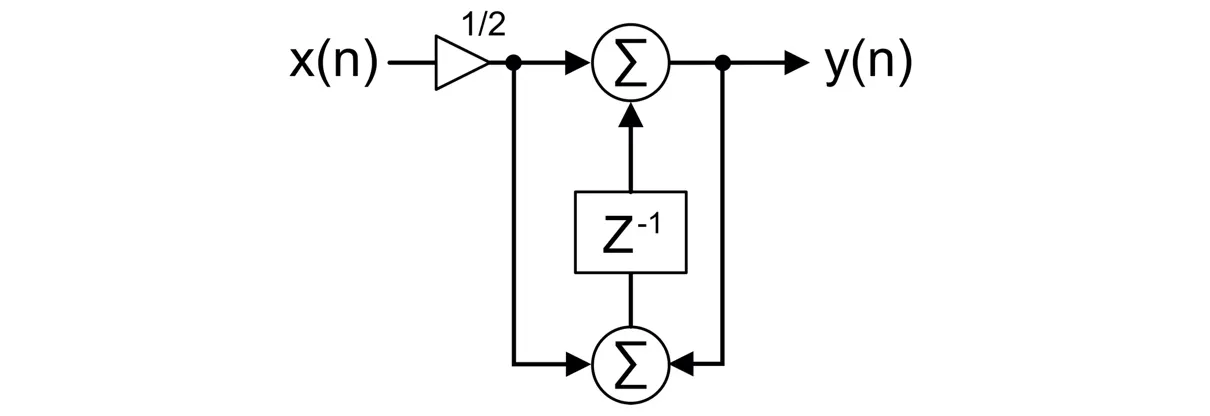
By balancing the forward and reverse integration step functions, this architecture produces an interpolation that better approximates the real signal.

A one-pole filter

To turn this integrator core into a one-pole filter, we simply need to make the integrator leaky, just like we did for the simple one-pole filter at the start of this chapter. We can do this by subtracting the integrator output from the input and scaling it by an appropriate coefficient.

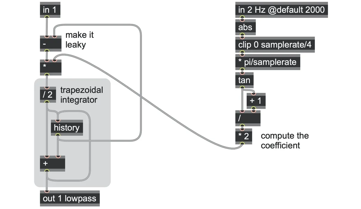
You might notice that this bilinear transform version requires a slightly different formula to convert the desired cutoff frequency in Hz to the multiplier coefficient compared to the one pole filter we saw at the start of this chapter. The reason why is mathematically beyond the scope of this book, but has to do with counteracting a certain warping of the frequency range that the bilinear transform implies.[60] This change also means tht we can only use cutoff frequencies up to one-quarter of the sample rate (a 12kHz limit at a samplerate of 48kHz), here ensured using a clip operator. We can also simplify this patch slightly by rearranging and noting that the * 2 and / 2 operators cancel each other out.

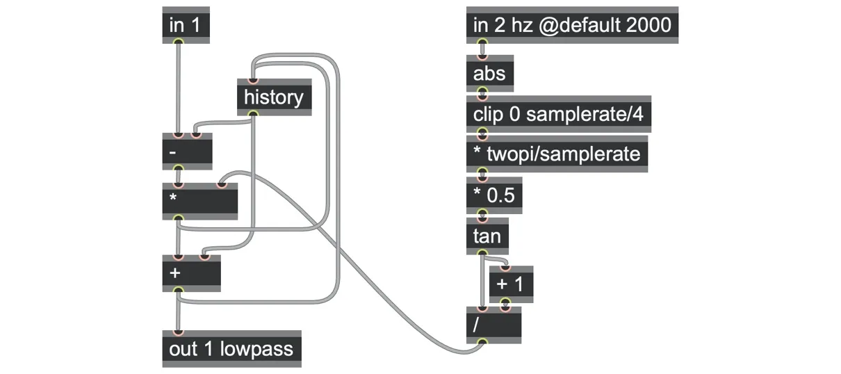
The trapezoidal architecture allows block diagram designs that more closely resemble analog circuit designs. That is, the trapezoidal form of the one-pole filter here is much closer to the ideal form of a blend between the raw and filtered signal (which is otherwise impossible due to there being ideally no delay), with better phase response, and thus a better approximation of what an actual analog resistor-capacitor circuit should produce. Another advantage is that the implementation is very stable and handles quite extreme frequency modulations up to audio rates very well.

As with the naïve one-pole filter, we get a free highpass filter by subtracting the lowpass from the input (and, with another subtraction, an allpass filter).

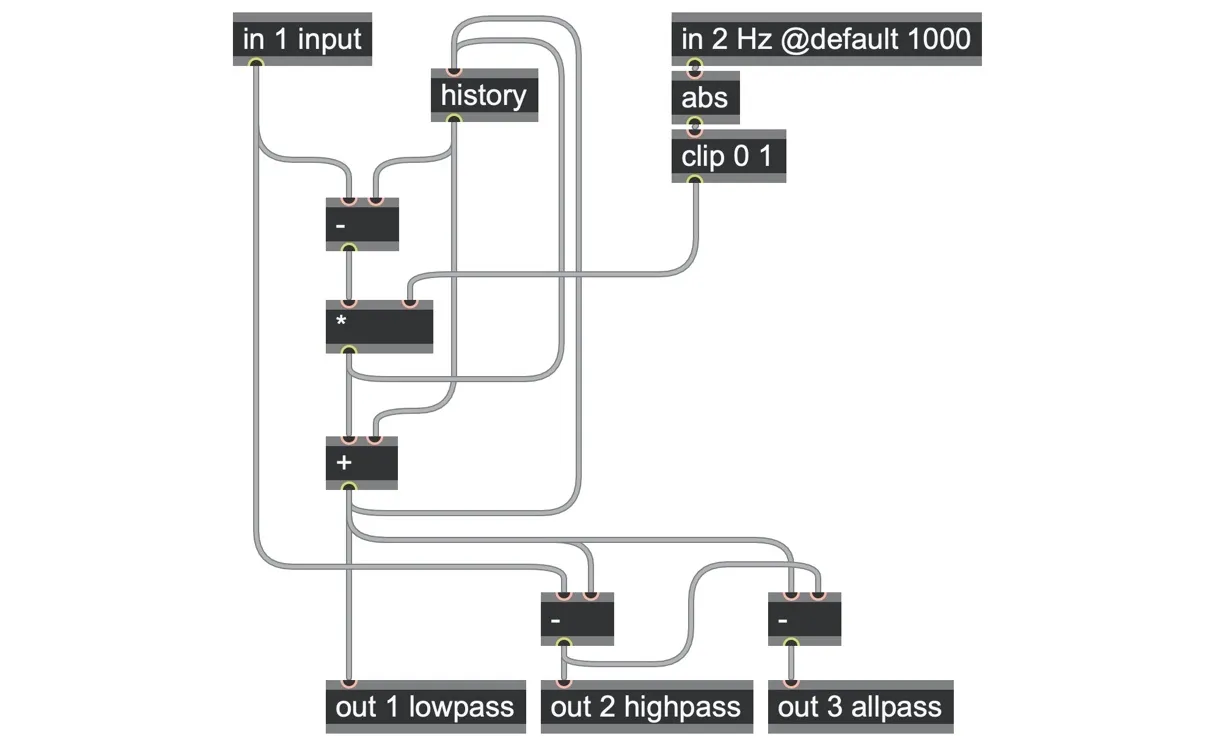
go.onepole.hz.gendsp

State Variable Filter

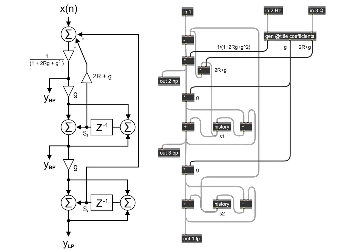
From this trapezoidal filter core, we can also build up many other filter structures fairly easily and at less computational cost than direct form biquads. For example, by nesting just one additional trapezoidal core, we can construct a "state variable filter" (SVF: a filter that produces many different spectral shapes at once) simply by tapping the circuit at different points.

Here is the block diagram together with our gen~ operator translation of it:

Here is the “coefficients” subpatch:

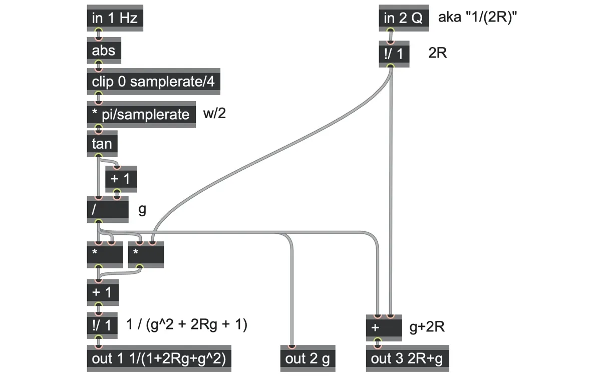
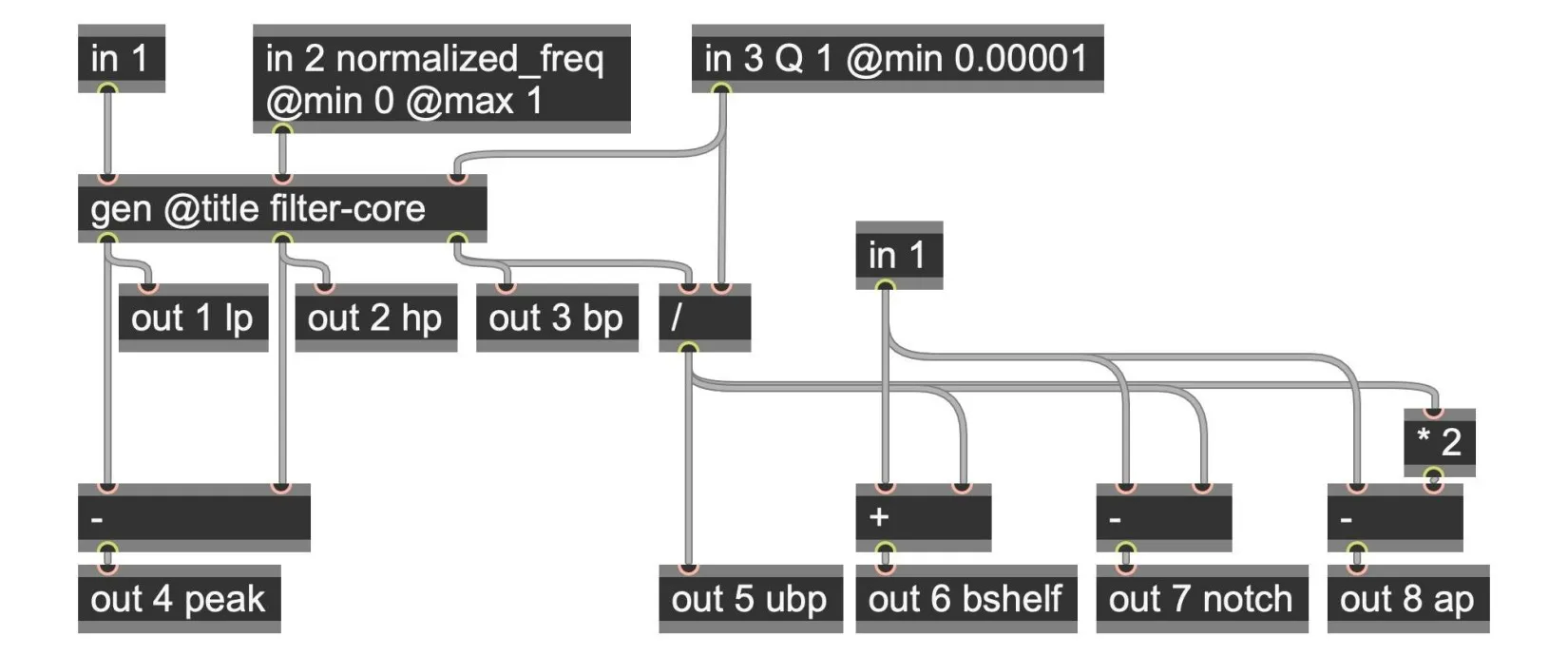
Note that, unlike the biquad, we don't need to compute new coefficients for each of the filter shapes–they are all produced simultaneously. Moreover, we can also derive several other filter shapes from this patch, including a peak, two different bandpass filters, a notch, and another allpass filter. These additional shapes come at almost no computational cost, using fewer components than a biquad, and without needing to compute any new coefficients.

go.svf.gendsp

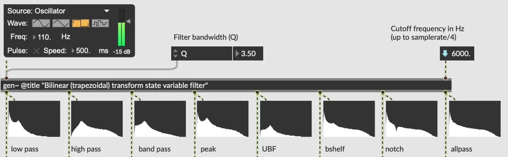
trapezoidal-state-variable-filter.maxpat

Crossover filter

Sometimes we want to split a signal into different frequency ranges and then treat the two outputs separately — spatializing or compressing them differently or splitting the signal to build a simple equalizer. You might assume that splitting a signal into two ranges could be done by passing a signal through both a lowpass filter and a highpass filter, but it's not quite that simple. If you try adding the lowpass-filtered and highpass-filtered signals back together, the result sounds somehow still colored compared to the original source. The reason for this is that when we put our original signal through the two filters, each one adds different phase delays that interfere with each other when mixed back together.

We can work around this problem by inserting an allpass filter that uses the same frequency parameter as the lowpass filter, in order to compensate for the phase delay. That is, if we split a signal into two paths, feeding one path through a lowpass to shape the sound and the other path through an allpass (which doesn't shape the sound but applies the same phase delay), we can then mix the two resulting signals without any distortion. And as we saw in the last section, this also means we can get a highpass filter simply by subtracting them.

But what kind of lowpass filter would we want, and what works? We don't want a resonant filter for a clean crossover, and we know a one-pole filter doesn't resonate. Although a regular allpass doesn't have the same phase response as a single one-pole lowpass filter, it does happen to have the same phase response as two one-pole lowpass filters in series.

So, let’s feed our audio input into both a chain two onepole lowpass filters, and subtract them from allpass filtered copy of our input, to create our two phase matched crossover signals.

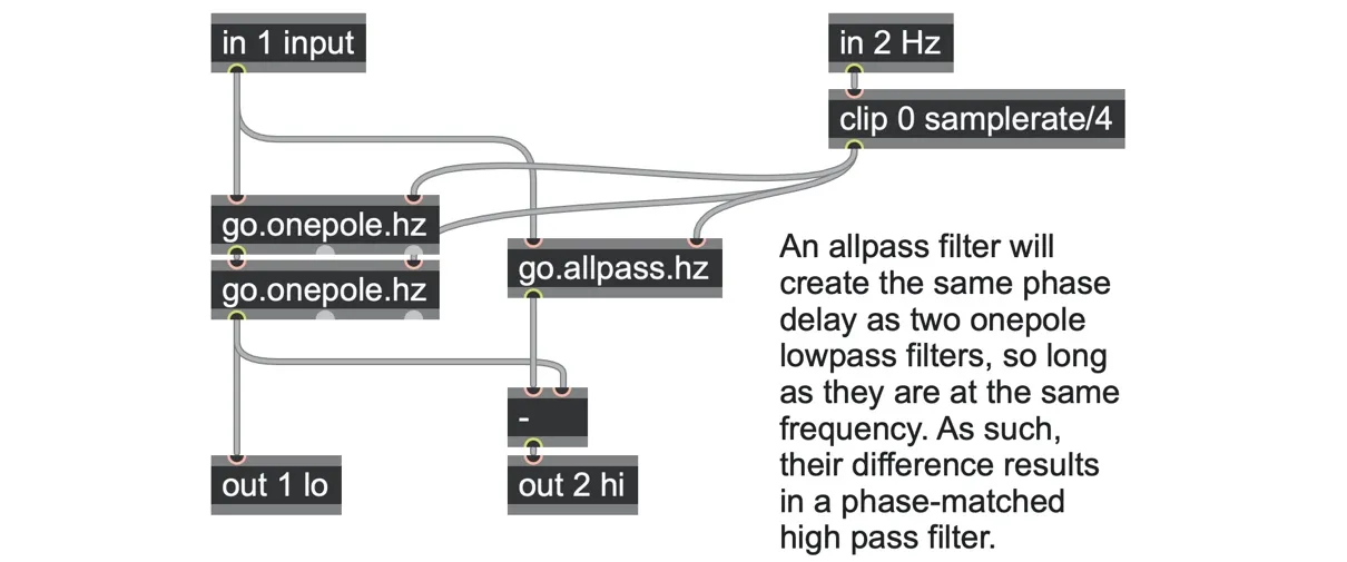
crossover_simple.maxpat

This method of creating a crossover filter can be expanded further to increase the number of frequency-band channels. All you need to do is ensure to add matching allpass filters to each remaining channel in order to preserve the total phase delay. Here is an example of a three-band crossover filter.

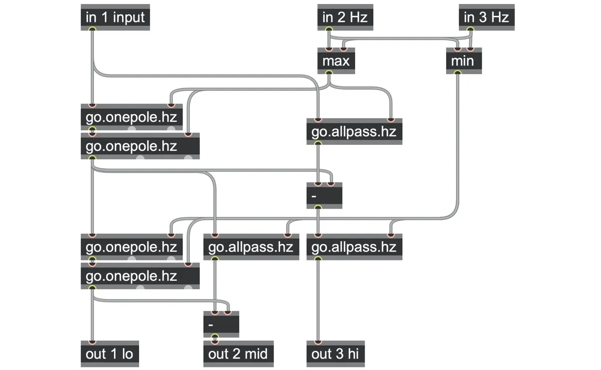
crossover.maxpat

Block diagrams: between theory and practice

As you go off in search of block diagrams that you might like to try implementing in gen~, here are a few suggestions you might want to keep in mind.

It is often not enough simply to copy a block diagram and start patching from there; you may need to spend some time reading through the source from which you copy the block diagram. For example, block diagrams are sometimes meant to provide conceptual models rather than a starting point for implementation. One obvious place you may notice this is a situation where you realize that your block diagram has a feedback loop with absolutely no delay — which is simply not possible in the digital world. It is often the case that reading further into the text will reveal how the problem is resolved.[61]

Or, you might encounter a block diagram symbol whose meaning isn't as well defined. For example, you might run across the Integral symbol ( ∫ ). That can be a tricky one to encounter since it might mean a simple integrator (which would be a simple substitution using the accum operator), but it might also mean that you need a "leaky integrator" (as we have seen with lowpass filters), or it might be a conceptual indication of an "impractical" filter. You may need to go beyond the block diagram into the text to figure out what you need.

Finally, it's also sometimes the case that the way that a block diagram describes signal flow isn't actually the way that most algorithms do the calculation. We've already made a few changes to block diagrams in the patches in this to make them easier to read, and sometimes more efficient.

Smoothing control signals with lines and slews

We mentioned earlier that a one-pole lowpass filter can also be used to smooth out noisy or steppy control signals (and that's exactly what the slide operator does), but it's not the only way to do this and not always the best choice. As we saw with the lowpass gate, the one-pole approaches its target exponentially, starting off quite quickly and getting slower as it closes the gap with each passing sample frame. This varying slope isn't always desirable, nor is the fact that an exponential approach never actually quite reaches the target. Here we'd like to introduce a couple of alternatives that maintain a constant slope and do reach their targets.

Limiting a slope (slew limiting)

One simple way is to limit how much change can happen on any sample frame, which means limiting how steep a slope can ever be. This is known as a slew limiter, and it will turn any stepped signal into one with smooth ramps between the steps. We can think of this as a kind of constrained motion. Here we'll use a history operator to store our current position, and we can compare this to the input target to find out what direction we need to go to meet it. If we then limit this difference to a maximum positive or negative amount using a clip operator, we can set the maximum movement our line can take in one sample frame. Adding that movement to our history position takes us a little closer to the target, and this is fed back to update the history for the next sample frame.

This is such a handy little circuit that we created abstractions for it, including one in which you can set the maximum rising slope independently of the maximum falling slope (very handy for creating a basic envelope from a gate signal):

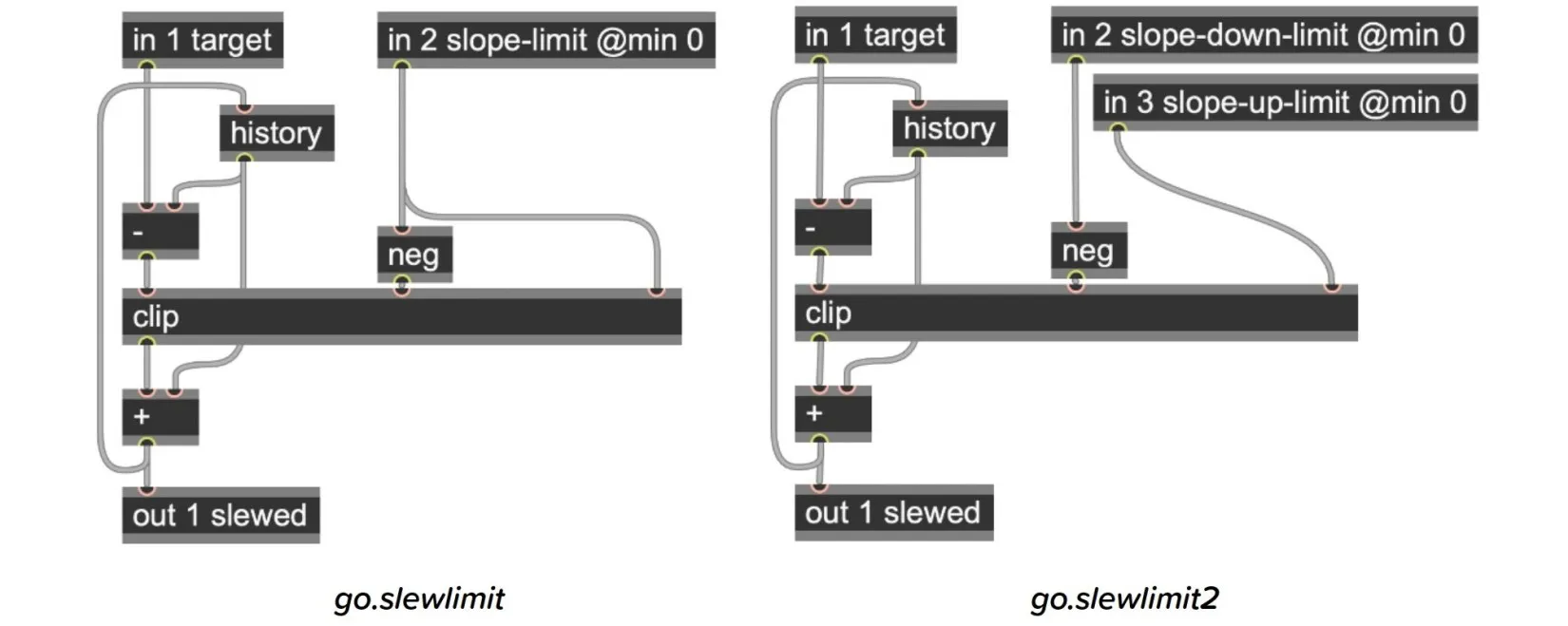
The slope-limit inputs specify the maximum rate of change per sample frame. That might not be the most intuitive form, but it is easy to compute a unipolar ramp slope as frequency/samplerate or, more generally, to specify a slope in terms of a duration in milliseconds using a !/ 1000/samplerate operator.

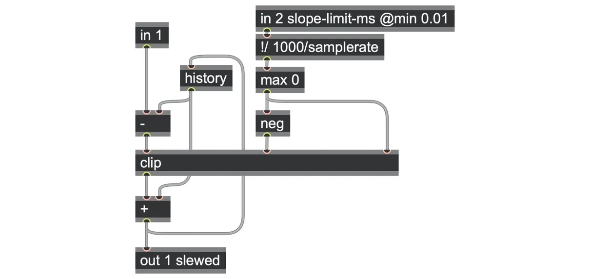
go.slewlimit.ms

Drawing a line (lag generator)

A slew limiter will take a longer time to cover a larger distance or a shorter time to cover a shorter distance, but that's not always what we want. Sometimes we simply want to be able to trigger a ramp from one point to another, somewhat like the Max or RNBO line~ object.[62]

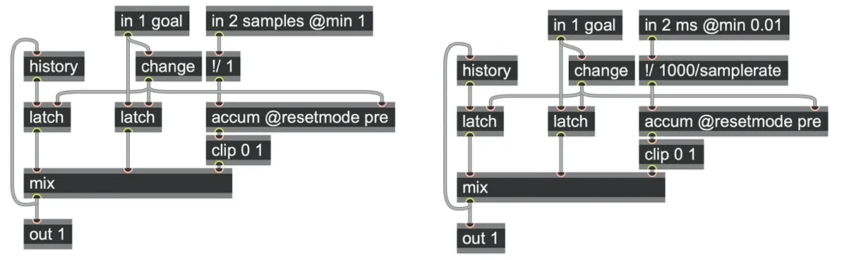
As we saw with the "smooth-stepped" circuits in Chapter 3, we can create linear glides from 0.0 to 1.0 over a fixed duration using an accum and a clip 0 1 operator. The first inlet of the accum operator sets how quickly it will rise (the slope per sample frame), which we can compute as 1 / duration in samples, just like any phasor ramp (or we could set using Hz or milliseconds just like we did for the slew limiter in the last section). Any non-zero trigger to the accum operator's second inlet will restart the ramp from zero again.

The "smooth-stepped" circuit from Chapter 3 can generalize this 0.0 to 1.0 ramp to any start and end point. We'll again start from a history operator that represents our current location and an input representing the goal we want to reach. We can restart our accum ramp whenever this target changes, using a change operator. At this moment, we can use a couple of latch operators to capture the current value of the input as well as our current location. Then we can simply use a mix operator to create a linear path between these two points, where the blend factor is simply our clipped accumulator. (You can also experiment with adding unit shapers to the clipped accumulator here to create nonlinear paths.)

go.line.samples and go.line.ms

The smoothing filter we've created here is also known as a "lag generator": it will try to replicate the signal at its input, but with a certain amount of delay in catching up to it. If the goal changes mid-ramp, that's not a problem. The change operator will cause the first latch to capture the start point as wherever we currently are, and the new endpoint as the changed input, and a new ramp will start. But there's one important subtlety here: we used accum @resetmode pre here to ensure that even on the first sample frame in which a change occurs, the ramp has already set off in motion. (If we didn't do this and just used a regular accum operator or accum @resetmode post, then the ramp will be at 0.0 whenever the input changes. With a continuously changing input, the ramp would never move away from 0.0, and so neither would our output.)

Finally, here are three control signal smoothing methods compared in the slide_slew_and_line.maxpat patch, using the same stepped signal as input. Notice that with go.line, the duration of each ramp is the same, but the slope differs. With the slew limiter, the slope is nearly always the same, but the duration can differ.

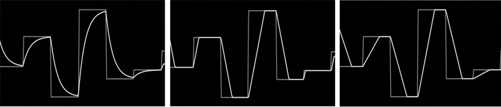
go.onepole	go.slewlimit	go.line