Appearance
Chapter 3:
Unit Shaping
In Chapter 1, we saw how useful it can be to think about ranges of values and how we can use a scale operator to transform between one range and another. Internally, the scale operator first maps the input to a unipolar (0.0 to 1.0) range and then maps that unipolar value to the desired output range. This is an example of why the unipolar range is so useful as a kind of common intermediate format for many kinds of transformations. In the last chapter, we also saw how changing the slope of a unipolar ramp can be so powerful for articulating timing.
We also talked about the importance of thinking about the shapes and curvatures of signals–which can impart a great deal of the expressive character of melodic glides, envelopes, and other dynamics, as well as the timbre of audio. In this chapter, we'll be looking at a variety of functions to apply shapes and curvatures to unipolar signals and a few of the ways they can be useful. We call these functions "unit shapers." Briefly, here are some of the many ways they can be used:
To change a robotic metric tempo into one with swing.
To create more interesting oscillator and LFO shapes and morph between them.
To create more interesting interpolations, including animation-inspired easing functions, for natural slew and parameter movement.
To create a variety of interesting envelope shapes.
To apply waveshaping distortion to bipolar signals (especially audio)
To apply hard or smooth quantization (e.g., dividing octaves into scale or chromatic steps), as we see in Chapter 5.
To shape the distribution of a noise generator, as discussed in Chapter 4.
To apply window functions for granular and formant synthesis, explored in Chapter 10.
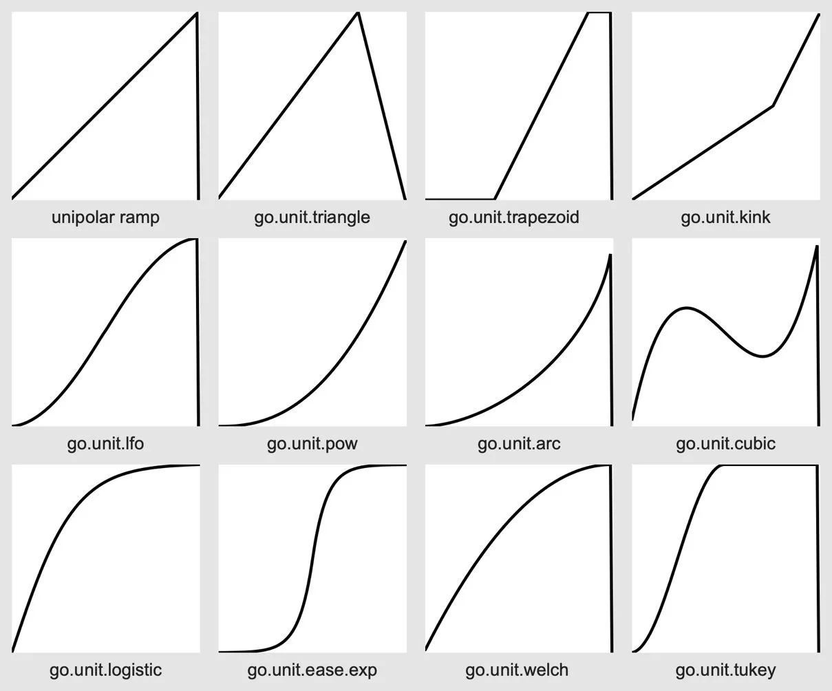
To be more specific, the term "unit shaper" in this book refers to any function that can take a linear input from 0.0 to 1.0 and produce at the output some other curved or nonlinear shape that still starts at 0.0 and ends at 1.0. We built a collection of unit shapers in the repository of patches included with this book, all prefixed with "go.unit". Some of these shapers also take additional parameter inputs to further control their shape.
Here are a few examples.
Swing and warping time
If we are working from ramp-based timing as we saw in the previous chapter, then we can use unit shaper functions to warp the time between beats to produce a variety of rhythmic effects, such as swing. In broad terms, adding swing to a rhythm usually means that every other ⅛th note (or half-beat) is delayed by some amount. Put another way; it means stretching and shrinking the times between the downbeat and the upbeat without changing the total duration between downbeats. Creating swing by unit shaping ramps doesn't just move the upbeats and downbeats; it also warps every other moment in between accordingly.
For example, let's use the go.unit.kink abstraction to break up a per-beat ramp into two line segments of different slopes. The go.ramp.kink abstraction makes these line segments that meet at a coordinate X and Y in the middle. The first inlet is for the ramp, and the second and third inlets set the X and Y coordinates, respectively (though the X coordinate is inverted by a !- 1 operator to make the shape work more naturally alongside other unit shapers).
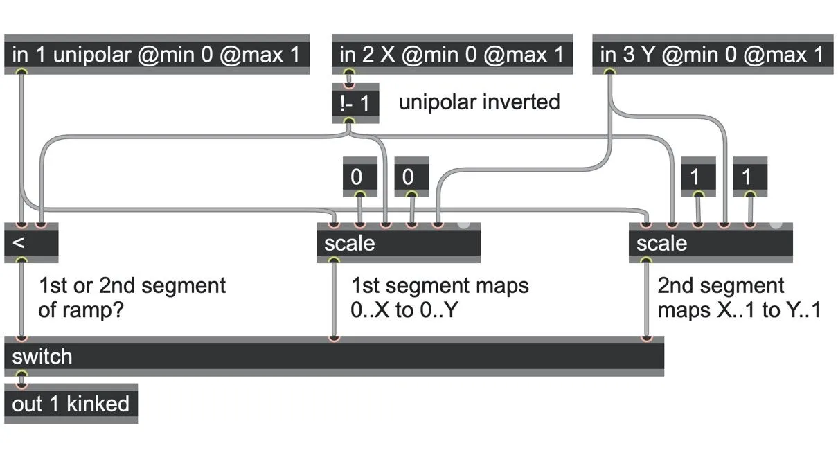
go.unit.kink.gendsp
It might look complex, but really, it's very simple. First, we check whether we are in the first half of the ramp (ramp < X) or the second half (ramp > X). For the first segment, the input range 0.0 to X is mapped to the output range 0.0 to Y, and for the second segment, the input range X to 1.0 is mapped to the output range Y to 1.0.
Let's plug that unit shaper into a BPM-based ramp generator along with a bipolar parameter param swing_bi to choose the intensity of the swing (so that 0.0 means no swing).
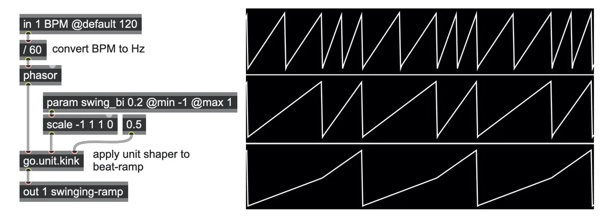
The bottom scope in the image above shows the kinked ramp per beat; the middle scope shows the ramp per half beat (revealing the swing action of delaying every other event), and the top scope shows the ramp subdivided by two, showing how it still follows the kinked ramp.
If we use different unit shaping functions, the time between each beat could be warped and curved in many different ways, each giving a different feel. For example, here are four different swing vibes:
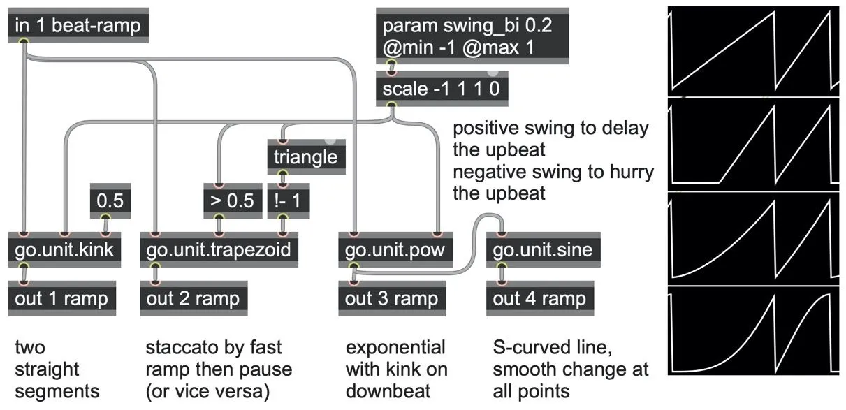
ramp.swing.maxpat
If we want to apply the swing warping to a ramp that spans multiple beats, such as a ramp-per-measure, we can use the general method of splitting a scaled ramp into steps and ramps using floor and wrap 0 1 operators respectively, applying the warping to the ramped portion only and recombining them through addition into a multi-warped ramp per measure (as shown in the bottom scope in the following image).
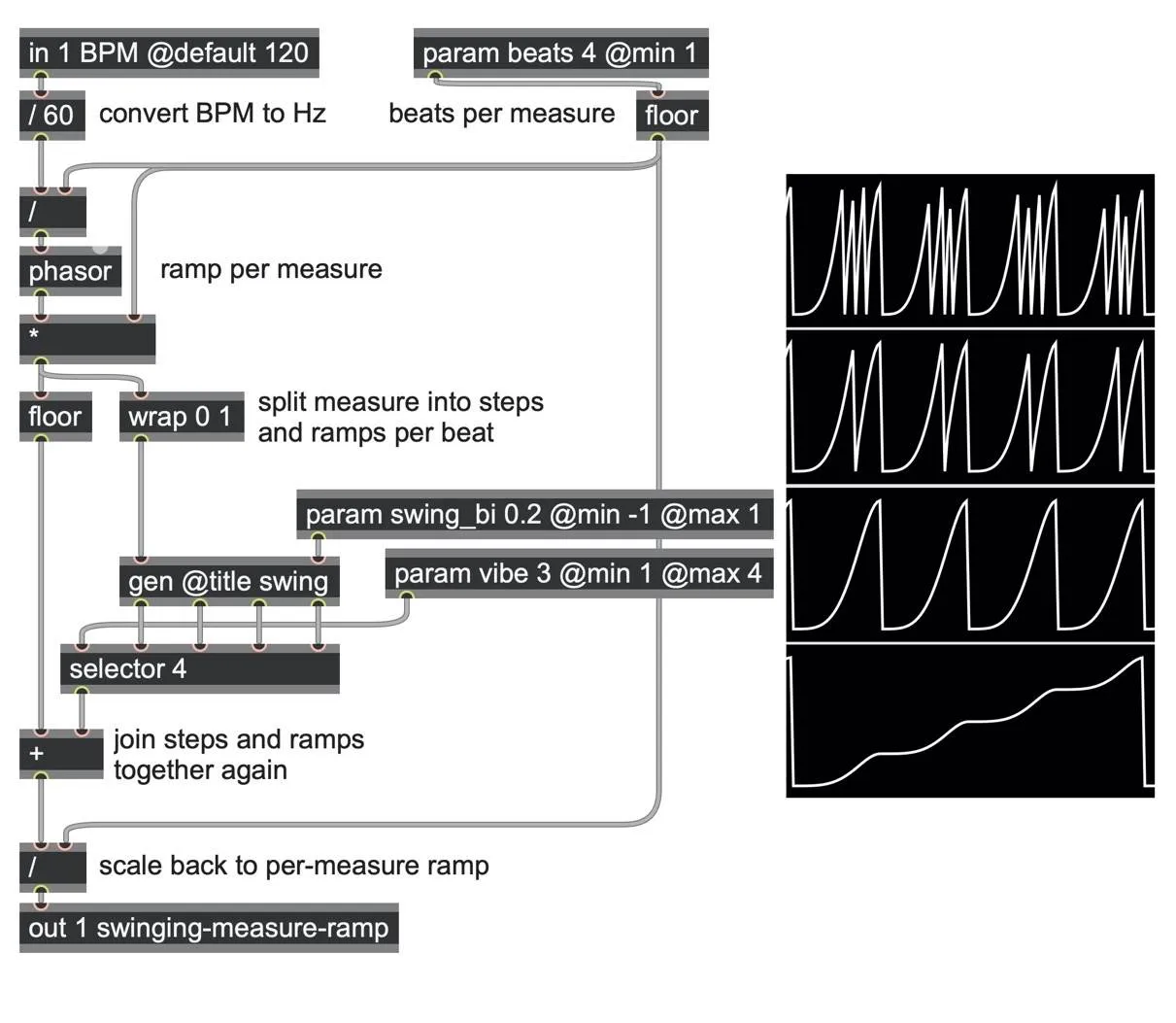
ramp.swing.maxpat
From ramps to LFOs
One of the great things about working with a common unipolar range is that we can chain one unit shaper with another to create more articulated shapes. Through the application of unit shapers, we can turn any low-frequency unipolar ramp into more complex LFO (low frequency oscillator) modulation signals.
Some of the most commonly used LFO shapes include rising and falling ramps, triangle-shaped waves, sinusoids, and square waves (or pulse waves with different duty cycles). In this section, we'll build up a simple LFO patch that uses a unipolar phasor ramp as the basic starting point, applying different unit shaping functions to build up many common (and some less common) LFO shapes. By controlling the unit shaper parameters, we can also morph LFO shapes over time. Moreover, if the input ramp is a tempo clock, then these will automatically be tempo-synced LFOs!
Triangles
Let's start with triangles. The triangle operator provides an easy way to convert a phasor ramp into several LFO waveforms. By default, it will map a 0.0 to 1.0 ramp input (left inlet) into a rising & falling triangle shape waveform, also in the 0.0 to 1.0 range. However, by changing the duty cycle parameter (right inlet), it can blend smoothly between a falling ramp, a skewed triangle, and a rising ramp.
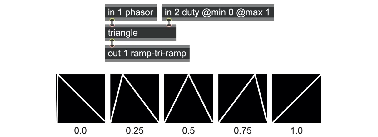
Looking carefully at the scopes, you may notice that with the triangle operator, the trough of the graph always remains in place, and the peak moves left to right as the duty input is changed. If you require the opposite movement (i.e., the peak remains in place, the trough moves right and left), you can use the go.unit.triangle abstraction, which routes a triangle operator through a scale 0 1 1 0 operator to turn it upside down within the unipolar range. For example, this may be preferable when using the triangle as the basis for envelope shapes.
You may notice that modulating the in 2 duty can quickly produce jumps or clicks in the output. This occurs if we are controlling the duty using a user interface such as a number box, which updates its values more slowly than audio rate, resulting in stepped changes of the waveform. But even some modulations at full audio rates can cause large value jumps that produce unwanted effects.
One way to solve these problems is by controlling when the parameter of the triangle operator is updated. Specifically, if we only update this control when the LFO waveform loops, the glitchy noise will disappear. Since the waveform loops when the input phasor ramp wraps around, we can use the go.ramp2trig abstraction we built in the last chapter and a latch operator to synchronize the parameter changes.
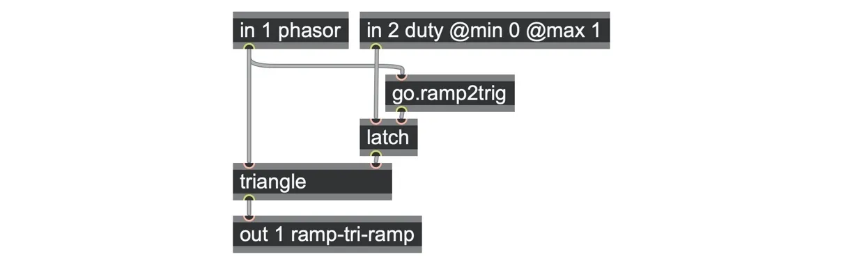
The latch will "sample" its left input when the right input is non-zero, such as when it receives a trigger from go.ramp2trig, and then the latch will "hold" that value until the next trigger (when the phasor next loops). You'll see this again in other patches in this book.
One of the nice things about using a triangle operator is that it has turned one unipolar ramp into a combination of two unipolar ramps (just that one of them goes down rather than up). That means any shaping that we could apply to a phasor ramp, we can also apply to our triangle output, and we can skew the result just by changing the triangle's duty parameter. It's great when we can produce several different outputs from the same circuit, and even better when it can continuously morph between them for almost no cost in complexity or performance! Now that we've got a morphing ramp-to-triangle generator, let's extend our patch to generate more LFO waveforms from the same circuit.
Sinusoids
Let’s start with sinusoids. We can quite easily generate a unipolar sinusoidal output from a unipolar triangle input by mapping through a simple mathematical function.
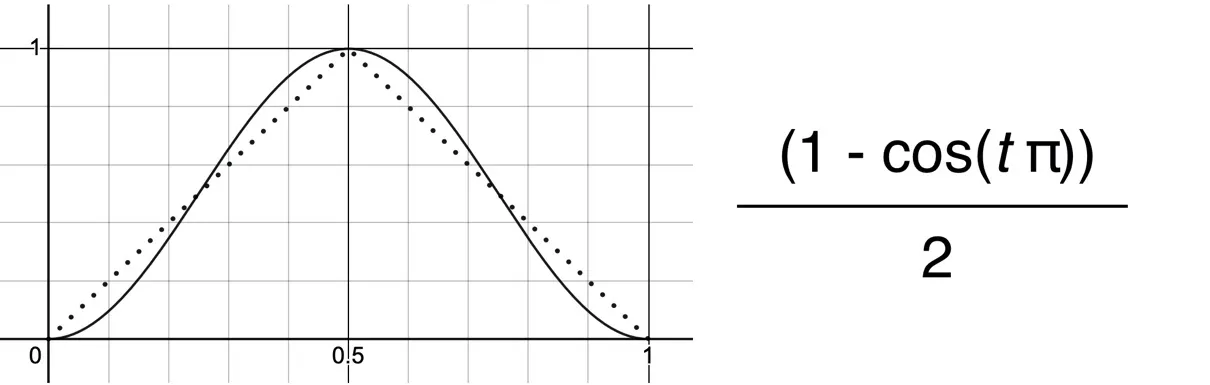
The dotted waveform is the triangle input “t”; the solid waveform is a derived sinusoidal function output: (1 - cos(t*pi))/2
As with most mathematical environments, the sin and cos operators expect angles in radians, which run from negative pi (-pi) to positive pi.[24] So, to compute our sinusoidal function as above, we can convert our triangle operator's output into radians using a * pi operator and then apply a cos operator. That already gives us a sinusoidal shape at the output, but it doesn't look similar to our triangle yet.
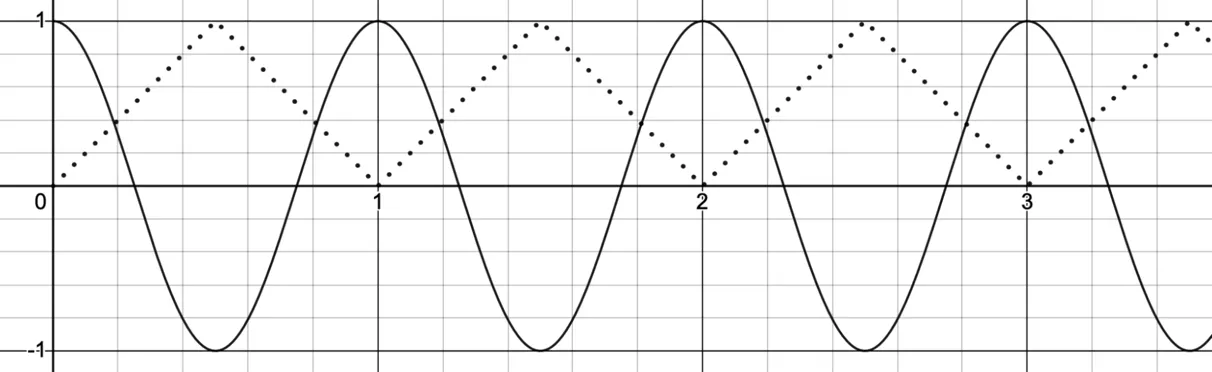
As you can see, the output of the cos operator is a bipolar signal between -1.0 and 1.0, but we want a unipolar output from 0.0 to 1.0. The cosine is also upside down relative to our triangle waveform (the peak of the triangle is at the trough of the cosine). Morphing between these waveforms would be more useful if they had the same direction.
In the mathematical equation above we corrected this by subtracting from 1 and dividing by two, but we got the same result in the following patch using a scale operator (scale 1 -1 0 1 both inverts the input and converts a bipolar signal into a unipolar signal).

go.unit.sine.gendsp
This trio of operators is a common need for unit shaping, and so we saved that as the go.unit.sine abstraction. Just remember — to get a full sinusoid out of this, feed it with a triangle wave.
Here we combined it with the triangle generator from the last section to get both triangular and sinusoidal waveforms with the same duty parameter.
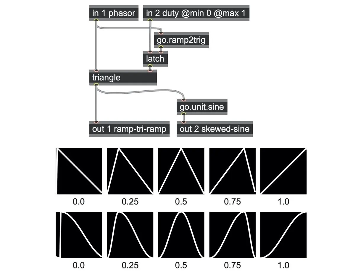
Now that we have both triangular and sinusoidal outputs, we could easily switch between them. But since we made our sinusoid have the same peak, range, and skew as our triangle, why not morph instead of switching?
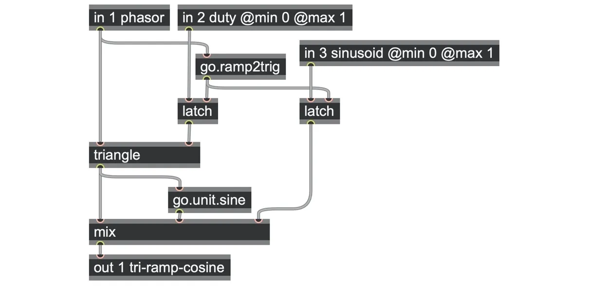
We can smoothly morph between the linear ramp/triangle output and the cosine waveforms by crossfading using a mix operator. To control this crossfade, we need another input (in 3 sinusoid in the following patch), and again we've added the go.ramp2trig and latch operators to make sure that it only updates the mix when the phasor wraps to avoid unintended clicks.
Pulse waves
Next, let's get a square wave/pulse output from our phasor ramp. A pulse wave is a logical signal–either +1.0 (true) or 0.0 (false)–and so naturally, we can use a logical condition such as a > ("more than") comparator operator to convert a ramp signal to a logical signal. For example, taking our original phasor through a > 0.5 operator will produce a neat square wave that is 0.0 for the first half of the period and 1.0 for the second half. As an alternative, we can pass the phasor through a - 0.5 operator to shift the phasor down by half a cycle and then test with a > 0 operator to see when the shifted phasor rises above the zero line.[25]
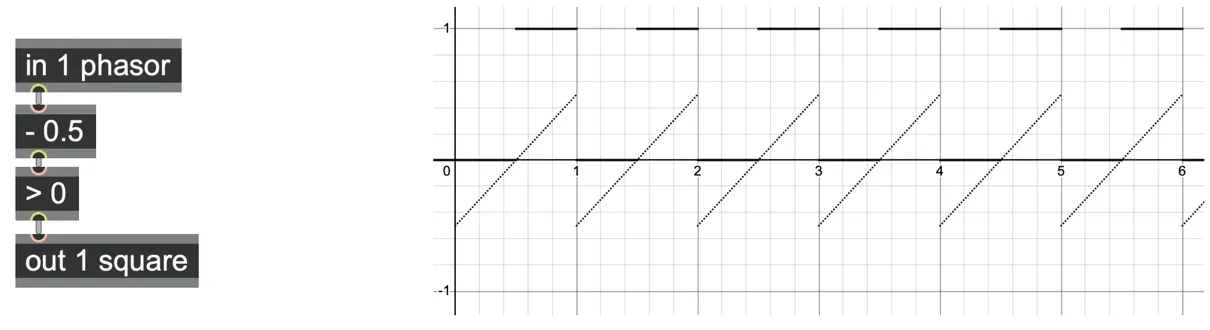
Dotted line: shifted phasor - 0.5; solid line shows the logical comparison > 0.
And if we change the argument to the subtraction operator, we will get different duty cycles. We could just map the param duty here to get variable pulse width, but it doesn't quite work the way we might like it to. As the param duty increases, the pulse width of the output decreases. We can fix that really easily just by sending the param duty value through a !- 1 (subtract from one) operator, which inverts the 0.0 to 1.0 range into a 1.0 to 0.0 range. Now when the param duty is 0.75, we get a pulse wave that is high for the first 75% of the period and low for the remainder.
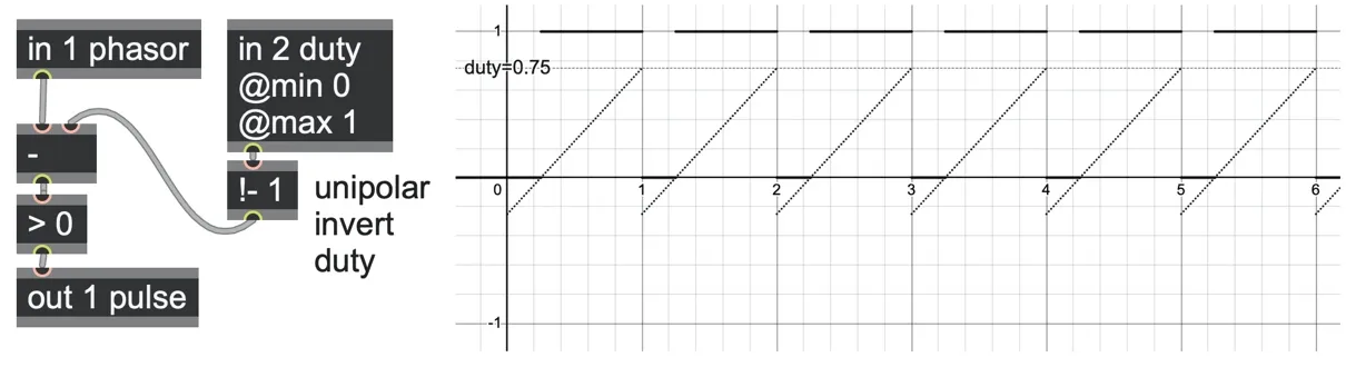
Dotted line: shifted ramp. Solid line: output pulse wave, with duty cycle (dashed line) = 0.75
In this way, we have built a pulse wave LFO with a pulse-width modulation (PWM) control due to the param duty operator.
Trapezoids
There's another neat thing we can do with our shifted phasor. If we multiply it by some number greater than one, we will make the slope get steeper. The bigger the number we multiply, the steeper it gets until it also starts to look like the pulse wave shape. Of course, this will also make it burst beyond the 0.0 to 1.0 range, but we can fix that very easily by sending the result through a clip 0 1 operator. Finally, we can also recenter the phasor after this multiplication, simply by adding back on the inverted duty we had subtracted. The result of these changes is a trapezoidal wave.
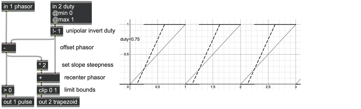
Dotted line: input ramp. Solid line: pulse wave with duty cycle = 0.75. Dashed line: trapezoidal waveform, using a multiplier of * 2.
You might notice how the trapezoidal waveform connects the middle of the bottom pulse wave segment to the middle of the top pulse wave segment. If the multiplier was * 4, then it would blend from a quarter of the way into each segment. The bigger the multiplier gets, the steeper this line becomes until it begins to look just like the pulse wave. And, going the other way, the closer the multiplier gets to 1.0, the more it begins to look like the original phasor. We now have an algorithm that can smoothly morph between ramps and pulse waves!
It would be neat if we could control this morph with another unipolar parameter, such as an in 3 shape @min 0 @max 1 operator. All we need is a bit of math to neatly compute the multiplier from the in 3 shape. The smallest multiplier we could use is 1.0, which leaves the ramp unchanged. The largest multiplier we could imagine would be something almost infinite, which would turn the ramp into a step. There’s lots of different math functions that can map a range of 0.0 to 1.0 into a range of 1.0 to infinity; here we’ll use the simple expression 1.0 / (1.0 - shape); which we can achieve very compactly using a scale 1 0 0 1 -1 operator.
There's just one catch: We can't actually compute the infinite slope when the in 3 shape is exactly 1.0. But, in this case, our trapezoid would be exactly the same as a pulse wave, so we can simply use a switch operator accordingly.
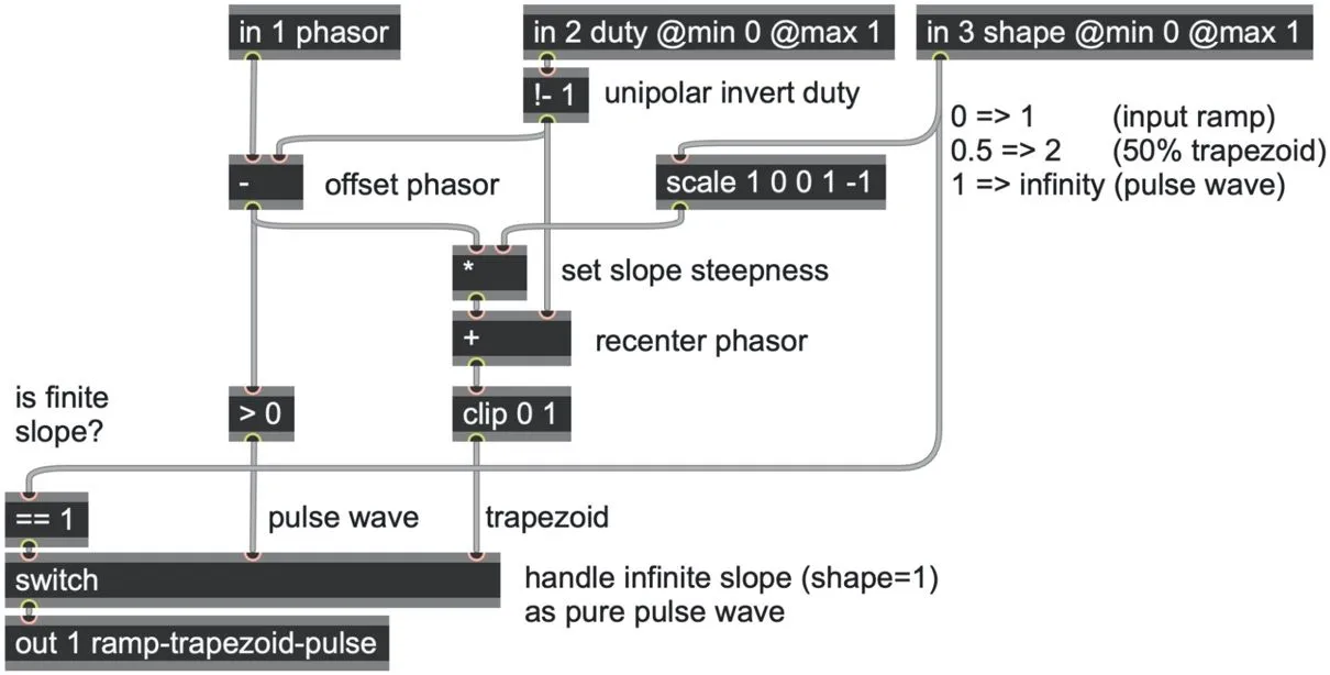
go.unit.trapezoid.gendsp
We now have a pretty simple function that can morph from a ramp, through a rising trapezoid ramp, to a pulse, and we can modify the pulse width duty cycle of them. We saved this as the go.unit.trapezoid abstraction. To get a trapezoid that can both rise and also fall, all we need to do is feed the go.unit.trapezoid abstraction with a triangle wave, whether from the triangle operator or from a go.unit.triangle abstraction.
Moreover, when the trapezoid shape input is zero, it passes the triangle through unchanged, so we can also combine it with the morphing to sinusoid from earlier to get an LFO that can morph between ramps, sines, pulses, and trapezoids, with a variety of intermediate shapes and duty cycles.
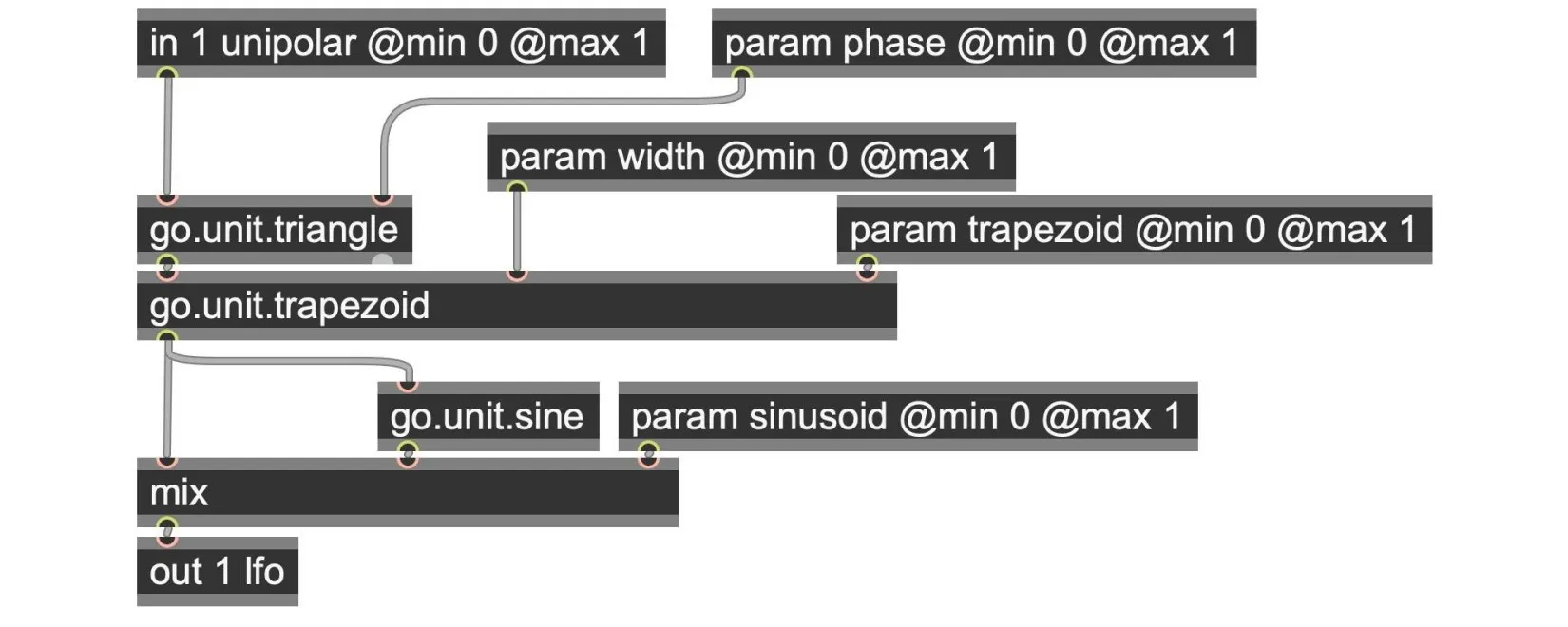
go.lfo.multi.gendsp
Here is a selection of some of the different waveforms we can get out of this patch:
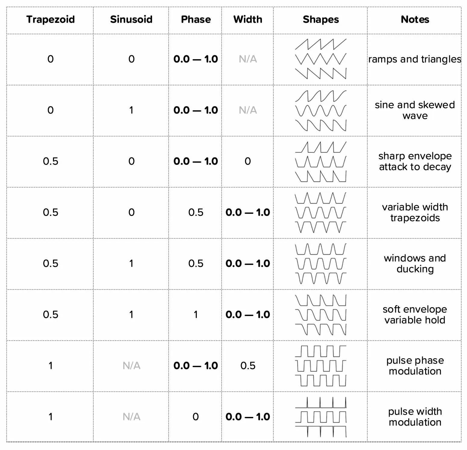
That's a very useful set of LFO waveforms using very few operators and very few parameters. Moreover, we already know we can modulate the frequencies and phases of the input ramp using go.ramp.div, go.ramp.rotate, etc., and these will modulate the LFO output equivalently!
The output of all of these morphable waveforms are in the 0.0 to 1.0 range ("unipolar-normalized"), but sometimes we want a bipolar-normalized signal in the range of -1.0 to 1.0 for LFOs, just like audio signals. You can use a scale 0 1 -1 1 operator again here to do this or other scale operator inputs to map to any arbitrary range you need.
Shaping smooth-stepped interpolation for LFOs and smooth glides
In Chapter 1, we saw that a mix operator performs a linear crossfade from value A (first inlet) to value B (second inlet), according to a control parameter (third inlet). A linear crossfade is also known as a linear interpolator, as we'll explore in Chapter 6. Since the mix operator's control input expects a unipolar signal from 0.0 to 1.0, we can drive it with a regular phasor ramp, but more interestingly, we can also apply any kind of unit shaper functions to this ramp to create nonlinear crossfades and interpolations.[26]
To put this into practice, we're going to introduce a little "smooth-stepped" patching pattern that we reuse in many different patches in this book.
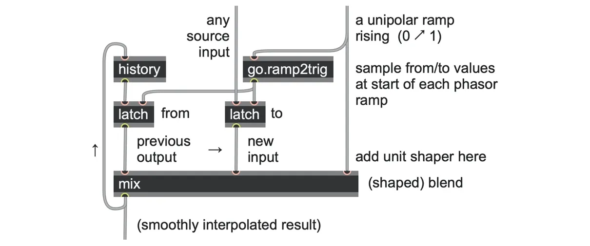
The core idea is to use a unipolar rising ramp (such as created by a phasor operator) driving a mix operator's control inlet to glide smoothly (interpolate) from one value to another. The target point of the glide is sampled from some external source signal–which could be anything at all–when the phasor wraps by using a latch operator and go.ramp2trig abstraction. The start point of the ramp is also sampled using a latch at the sample moment by taking the patch's own output, fed back through a history operator. In that way, the ramp always moves to a new position from wherever it was before.
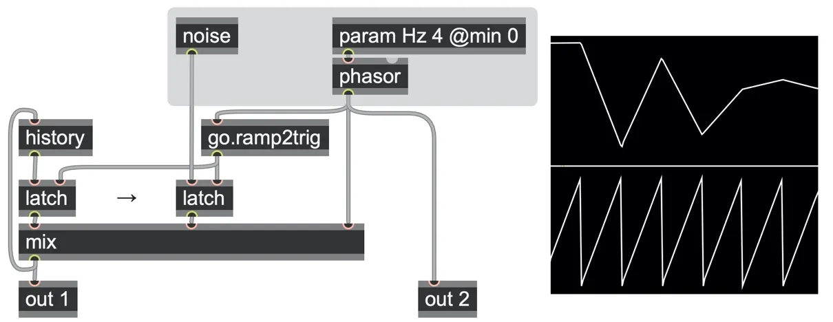
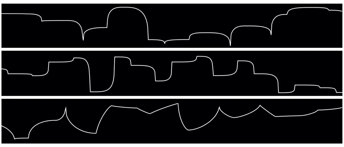
For example, by using a simple noise operator as the source signal, we will get a series of connected random glides, all synchronized to a driving phasor operator. We also added a second outlet to that patch, so you can see how the phasor output (bottom scope) drives the line segments of the main output (top scope).
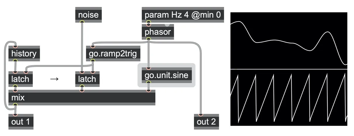
Since the driving phasor ramp always runs from 0.0 to 1.0, regardless of what the input and output signal values are, we can use any unit shaper to more interestingly curve our way between one value and another simply by inserting the shaper into the mix control. For example, we reused the go.unit.sine abstraction we built earlier in this chapter here.
LFOs from smoothed steps
We can use this to build another LFO by feeding it with a pulse wave that alternates between 0.0 and 1.0 with each ramp cycle. There are a few different ways we could do this, but to keep things simple and flexible, we're going to do it with a triangle shaper (go.unit.triangle) and simply invert the falling section of the triangle wave so that we get two rising segments.
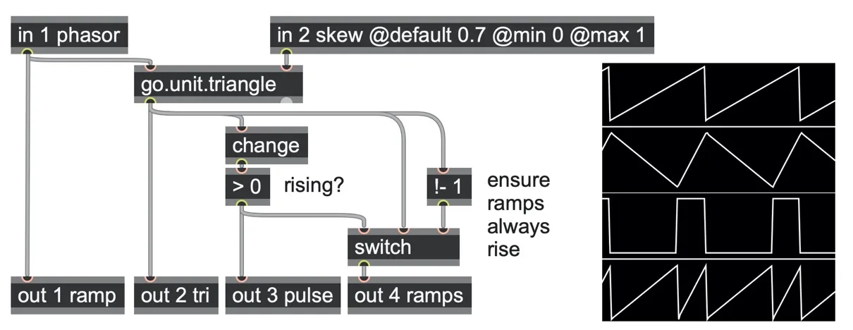
The change operator tells us if the triangle wave is rising (+1.0) or falling (-1.0). If it is not rising, then the > 0 operator returns false, and the switch operator instead routes a copy of the falling segment that has been inverted (turned upside down) via the !- 1 operator. In this way, our ramp segments are ensured to be always rising, which we will need for the smooth-stepping patch to work. As you can see, using the go.unit.triangle abstraction also gives us control over the pulse width via the in 2 skew operator. Let’s use this subpatch to feed our interpolator template and apply a unit shaper to the ramps before they reach the mix control input. Here we used the go.unit.arc[27] unit shaper, giving us another parameter to generate more interesting LFO shapes.
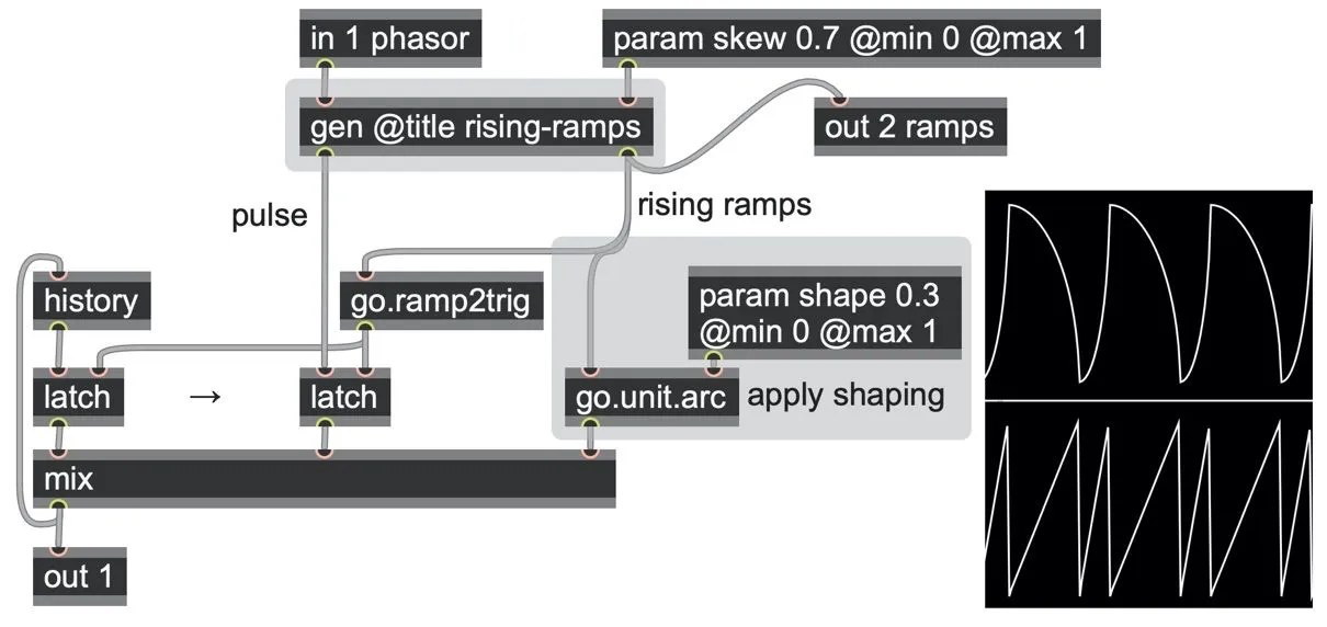
There’s a few more things we can add to this to open up more LFO shapes.
You might notice that the output has a somewhat “sharktooth” character in that the curvature is different whether the ramp is rising or falling. If instead you want a symmetric curvature, all you need to do is invert the shape parameter while the output is falling. We can tell if the output should be falling simply by comparing the two latches (the from and to values for the interpolation) using a greater-than-or-equal (>=) operator, and we can use that to drive a switch and !- 1 operator pair to do the conditional inversion, just as we did earlier.
We can also add a param symmetric operator to enable and disable this inversion through an and logical operator, so that inversion only happens if the ramp is falling and the param symmetric is enabled (non-zero).
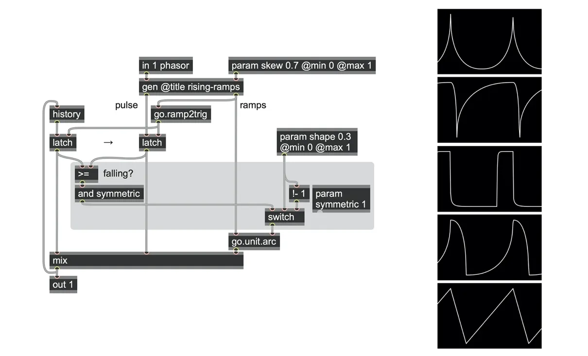
We don’t have to limit this patch to using only unipolar pulse wave inputs; we could take our input from any external signal using an in 2 operator.
We made this change in the next patch, as well as encapsulating the shape symmetry logic into the “symmetry” subpatch to keep things organized.
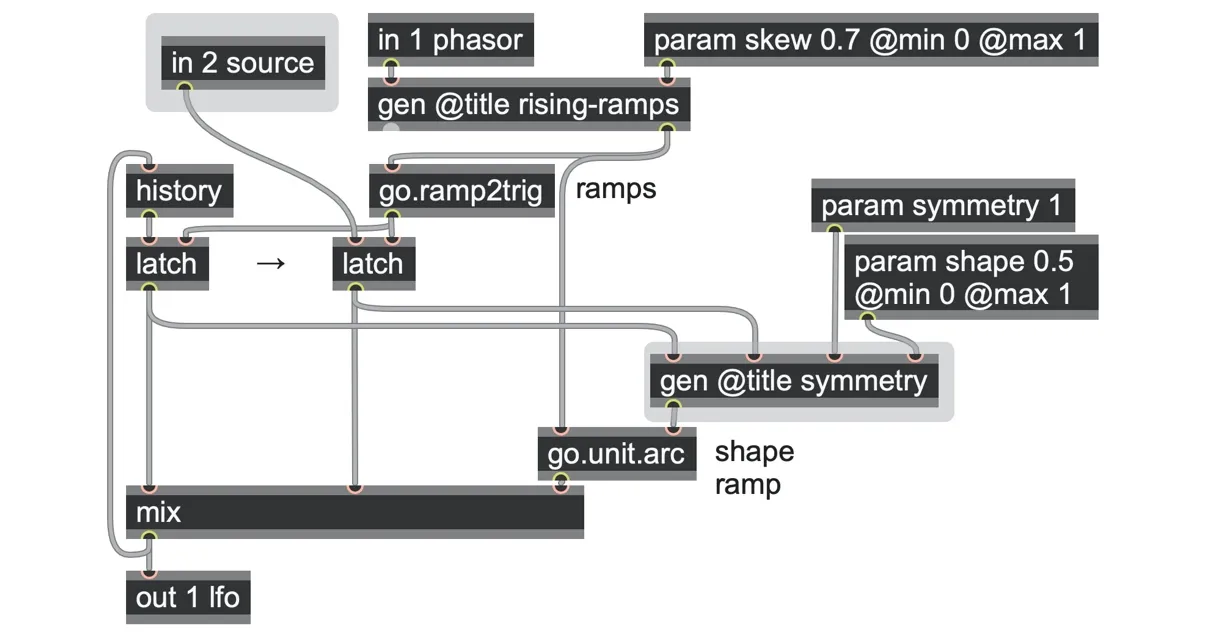
Here are some examples of the kinds of signals it can give when sampling from a bipolar noise generator. We’ll see more variants of this kind of smoothed stepped random generation in the next chapter.
Alternatively, we could strike a balance between our pulse wave and noise and between unipolar and bipolar. We could use another mix operator to blend the pulse with a little noise operator, made unipolar with an abs operator. Moreover, it’s very easy to convert the unipolar range of the pulse/noise mix to a bipolar range using a scale 0 1 -1 1 operator. We can put this under more dynamic control of a param bipolar by setting the lower output bound of a scale operator to either -1.0 (for bipolar) or 0.0 (for unipolar).
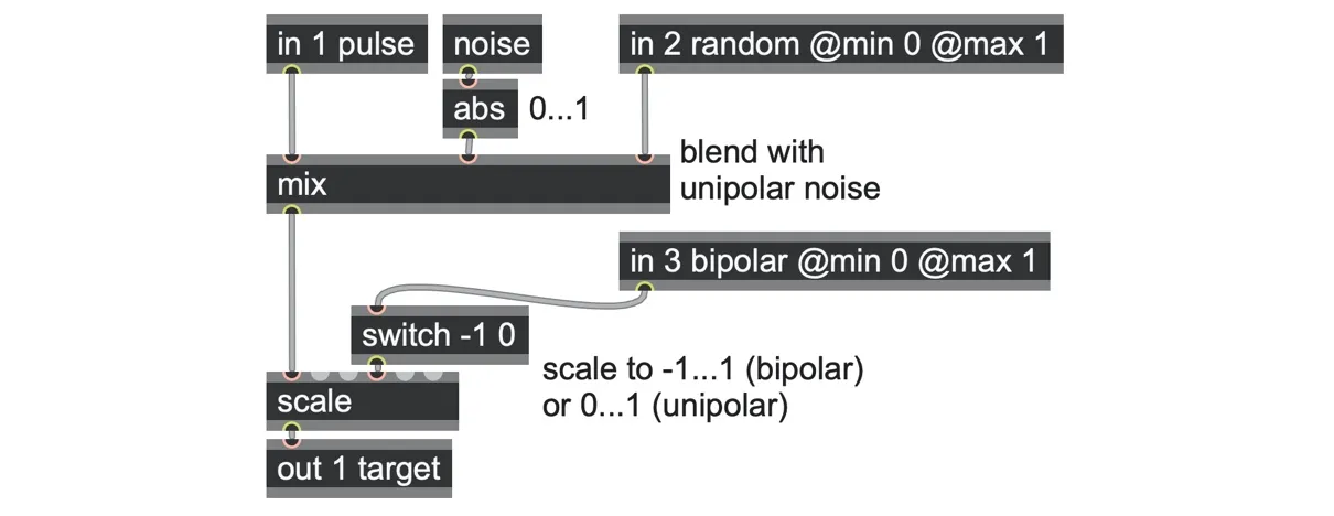
Let’s add this to our patch as a “target selection” subpatch. Finally, just as we did with our first LFO in this chapter, we can use a go.ramp2trig abstraction with latch operators to ensure that parameter updates only happen when the driving phasor wraps so that modulating parameters does not cause unwanted clicks. Here is the final patch with those changes added:
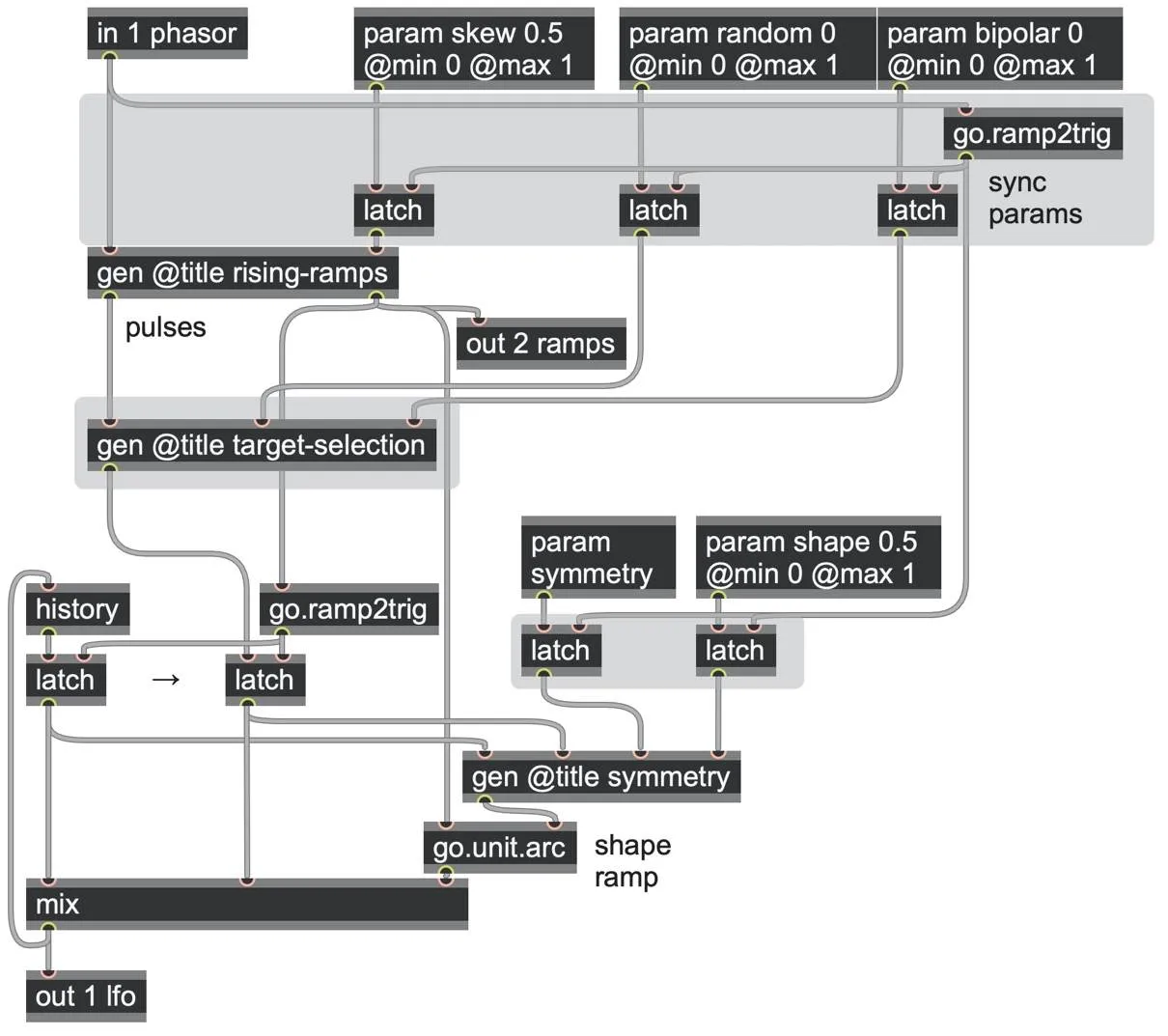
interpolating-LFO.maxpat
A slightly modified version of this patch is also available for your use as the go.lfo abstraction.
Glides and portamento
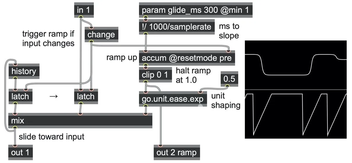
A phasor-driven smooth-stepped interpolator makes sense when you have control over repeating shapes. But we can use smooth-stepped interpolation for any arbitrary non-repeating input, to add for example smooth glides to sporadically stepped pitch changes. In this case, rather than driving the mix operator interpolator from a phasor, we can drive it from a “one-shot” ramp that is retriggered whenever the input changes.
As we saw in Chapter 2, we can easily create an endlessly rising ramp with an accum operator. If we want to stop it once it gets to a goal of 1.0, we can do that by sending it through a clip 0 1 operator. Any non-zero trigger to the accum operator's second inlet will restart the ramp from zero again. That gives us a "one shot" ramp that rises from zero to one and stops there.
This ramp can now smoothly interpolate between any two latch values by driving a mix operator just as we did before. The first latch operator represents our location when the ramp started, and the second latch operator is the target goal we are trying to reach. Whenever the input signal changes (as detected by a change operator), we can update these two latches and restart the accum operator's ramp from zero, to begin a new glide.
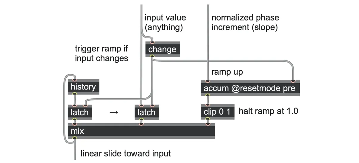
All we need to set the glide duration is a way to compute the required slope for the accum operator. For example, given a ramp duration in milliseconds, we can convert it to a ramp duration in sample frames using the mstosamps operator; and then take the reciprocal of that via a !/ 1 operator to get the slope per sample frame. Or, we can combine both of these operations into one using a !/ 1000/samplerate operator.
Now, whenever the input changes, we will begin a glide from wherever we are, even if we were mid-ramp, toward the new input value, and we always arrive after a fixed duration or "lag". In fact, what we have built here is also known as a lag generator, which we will explore in more detail in Chapter 6.
As with the smooth-stepped LFO, we can add a unit shaper of our choice before the mix operator’s control inlet to drive the curvature of the change. Notice how the ramp (in the lower scope) always rises from 0.0 to 1.0 and then holds there, regardless of what the input is:
For a more complex example with randomized curvatures, see the interpolating_glides.maxpat patch.
Easing functions
In the previous patch, the unit shaper we used is based on an “easing function.” Easing functions are drawn from a history of classic motions in animation, described in terms of three variants: an “ease in” that starts slow and speeds up, an “ease out” that starts suddenly but smoothly arrives at its destination, and an “ease in-and-out” that combines both for smooth start and arrival.
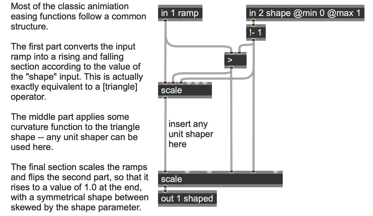
This book’s software repository contains several examples of common easing functions as unit shapers including go.unit.ease.pow, go.unit.ease.pow, go.unit.ease.exp, go.unit.ease.circle, go.unit.ease.back, go.unit.ease.elastic, and go.unit.ease.sine. For all of these we generalized the easing variants under a single “shape” parameter, where shape=0 means “ease in”, shape=1 means “ease out”, shape=0.5 means “ease in-and-out”, and any other value is a gradual blend between these. We'll use these easing function unit shapers in many patches throughout this book.
All but one of these follow a common patching template structure, as shown below. You can place any other unit shaper within this structure to create new easing functions.
Window envelope functions
A window function is a function that rises from zero to one, then falls back to zero, to provide the period and amplitude bounds of an event in a signal. In that sense, they are also a kind of envelope function. However, most often windows are symmetric in time.
We can create a symmetric rising & falling window shape simply by driving any unit shaper with a unipolar triangle wave:
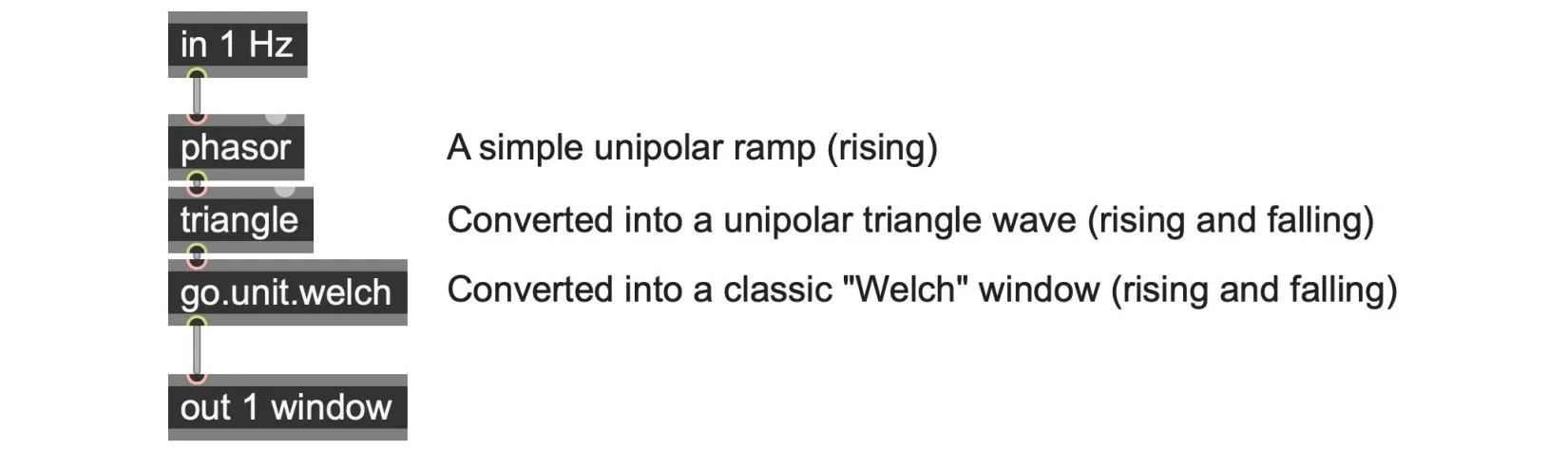
There are many window shapes used in signal analysis, granular synthesis, and related methods, and the book’s software package includes many of the most widely used as unit shapers, including go.unit.hamming, go.unit.hann, go.unit.blackman, go.unit.blackmanharris, go.unit.blackmannutall, go.unit.nutall, go.unit.flattop, go.unit.welch, and go.unit. parzen.
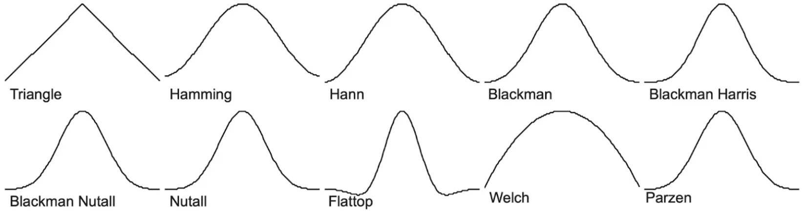
The software package also includes several widely used parametric window shapes, including go.unit.trapezoid, go.unit.tukey, go.unit.plancktaper, go.unit.gauss, and go.unit.raisedcosine.[28]
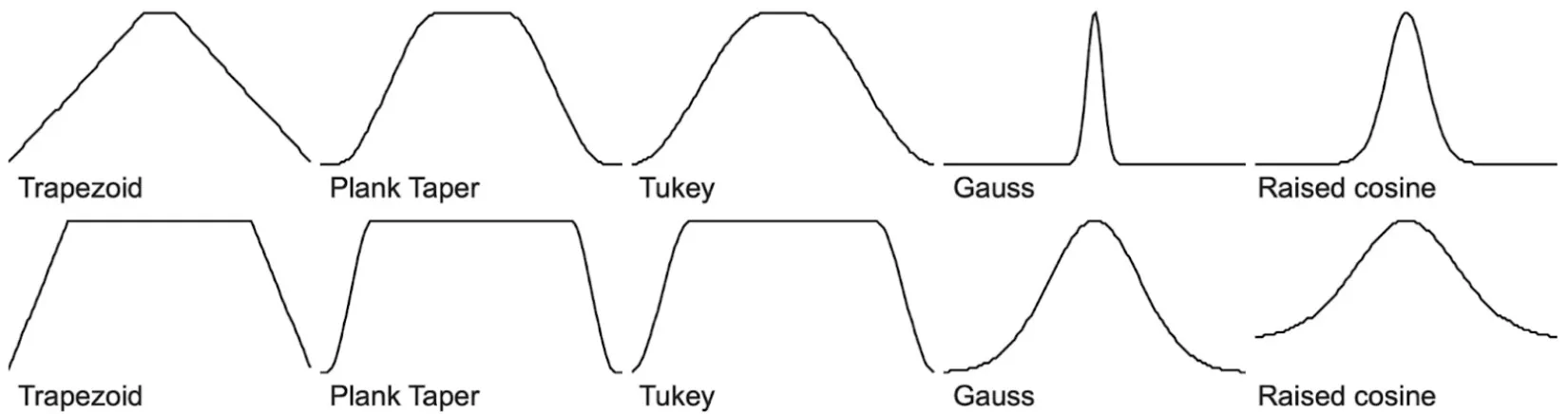
Of course, you can also use any other unit shapers for different windowing responses.
You can also create an asymmetric window or envelope shape simply by changing the second input of the triangle operator. For example, a triangle 0 operator will produce decay-only shapes. Or, you could extend the triangle operator into a trapezoid shape (such as generated by go.unit.trapezoid) for windows and envelopes with extended "hold" or "sustain" sections.
Waveshaping bipolar signals
So far, we have looked at ways of shaping based on unipolar inputs and outputs, but there are some specific cases–particularly when processing audio signals–where bipolar shaping makes more sense. This shaping of audio signals is often called waveshaping. It is a kind of distortion synthesis which can be useful to make a simple oscillator more complex, or to add soft limiting, overdrive, or other harmonically rich complexity to an audio signal.
We can build bipolar waveshapers from any of our unipolar unit shapers merely by applying a little extra patching to handle bipolar input and produce bipolar output. Here are two options:
Asymmetric: We could stretch the unit shaper over the whole bipolar range. Use a scale -1 1 0 1 operator to shrink the bipolar signal to a unipolar range, apply the unit shaper to this unipolar signal, and then stretch back to bipolar with a scale 0 1 -1 1 operator.
Symmetric: As an alternative, we can apply a symmetric mirror image of the unit shaper for the positive and negative signals. First, we take a copy of the signal and throw away any negative sign using an abs operator. This mirrors negative parts of the signal into the positive region, which is called full wave rectification. Then we apply the unit shaper to this rectified signal, then multiply the result by the sign of the input, so that the parts that were originally negative go back to being negative.
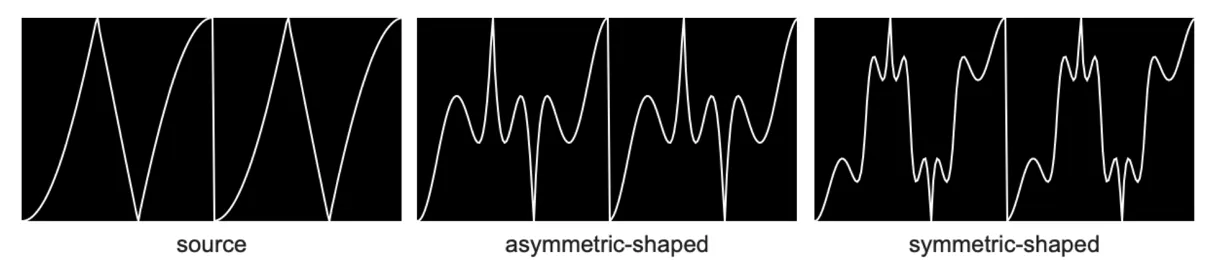
Both of these methods are shown in this patch, where we use a go.unit.spline unit shaper to make an input signal more complex.
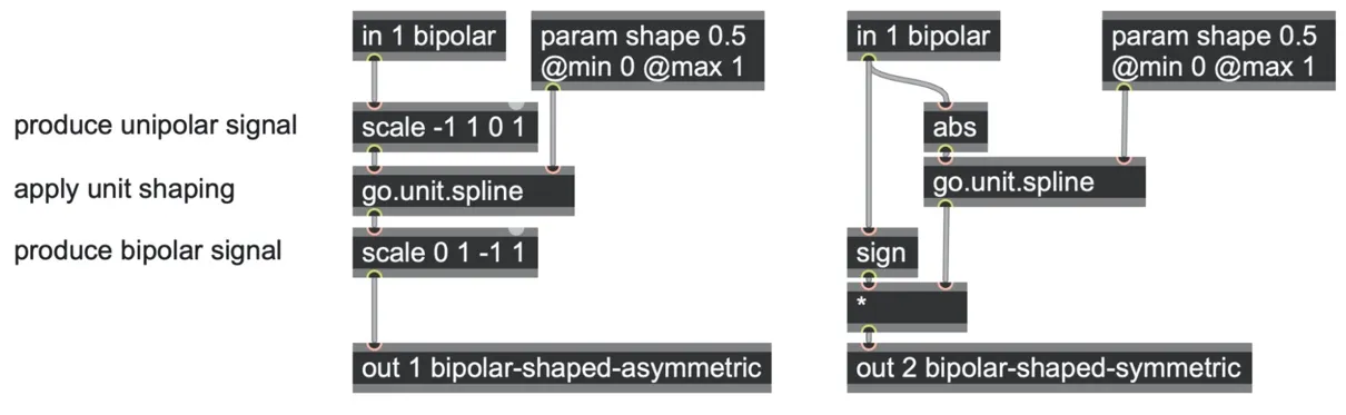
bipolar_waveshaping_unitshapers.maxpat
The results look like this:
Of course, you can use any input signal and any unit shaper–the following patch uses the go.unit.ease.pow shaper for example. Moreover, you can also easily explore a mix between the asymmetric and symmetric options if you wish:
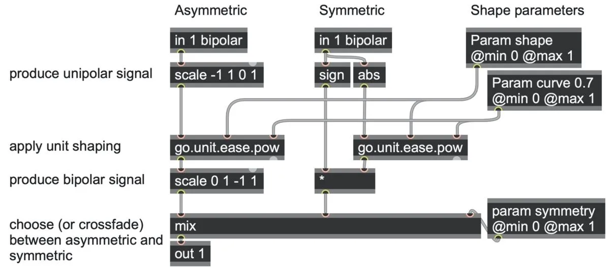
bipolar_waveshaping_unitshapers.maxpat
Audio waveshaping
As the last example showed, waveshaping can turn relatively simple waveforms into more complex waveforms. When processing audio signals, wave shaping imparts a timbral change to most input waveforms, and in this sense is comparable to filter-based signal processing (as we will explore in Chapter 7). However, there are a few interesting differences.[29]
Where most filters reduce the spectral complexity of a signal, waveshaping tends to increase it, adding more harmonics to the signal. For this reason, simpler waveforms such as sine and triangle waves are good choices for input. On the other hand, a plain square or pulse wave is not a good choice of input, as it has practically no slope in its waveform for a waveshaper to complexify.
Where the timbral response of most filters remain the same whether sounds are quiet or loud, the timbral response of a waveshaper is very dependent on the amplitude of the input: in many cases, the quieter the input, the less timbrally bright or complex the result. This correspondence of "louder" being "brighter" also tends to be the case for physically produced sounds, which means that waveshapers often respond in a perceptually satisfying way to enveloped inputs.
The specific effect of waveshaping on the spectrum of a signal is generally a nonlinear process, and for most shaping functions it is hard to predict precisely.
It can also sometimes produce harsh aliasing frequencies, particularly when using sharp piecewise linear shaping functions such as go.unit.kink and go.unit.trapezoid. Smoother functions of sigmoid, and polynomial, or sinusoidal nature are much less problematic. Let’s take a closer look at those.
Polynomial shapers
If you take a sine wave, and square it, you will get a waveform with twice the frequency (the second harmonic frequency). If you raise it to the power of 3, you will get a waveform with components up to three times the frequency (up to the 3rd harmonic). This continues for powers of 4, 5, 6 and so on.
Mixing an original signal with a slight amount of these power signals can be a relatively cheap way to add a bit of harmonic sizzle to audio. This is part of how exciter effects work. It’s also a relatively cheap way to create a kind of additive harmonic synthesis.
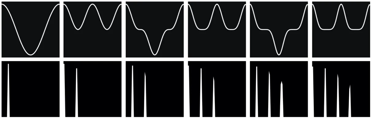
Top row: a sine wave raised to the power of 1, 2, 3, 4, 5, and 6.
Bottom row: the corresponding spectra showing the resulting frequency components.
We can mix these signals together, scaling each one by a different weight, to create a polynomial function. In mathematical terms, a polynomial just means a weighted mix of integer powers of the input signal x, and is notated as:
a0 + a1x + a2x2 + a3x3 + … etc. up to anxn,
or in code:
a0 + a1*x + a2*pow(x, 2) + a3*pow(x, 3); // etc
The degree of a polynomial is its highest power exponent (so, in the function above, the degree is 3), and this also tells you the highest harmonic it can produce from a sine input. So, if the input signal is a sinusoid, then the process above will have no frequencies higher than the 3rd harmonic.[30]
You may have noticed that raising a sine wave to a single integer power does not produce a single harmonic, but a mixture of harmonics. Unlike simple power functions, a special class of polynomial functions called Chebyshev functions produce only single harmonics from a sine wave input, so long as the sine wave is at unity gain. That is, if you feed them a sine wave of amplitude ranging from -1.0 to 1.0, they will output a single sine wave of a single higher harmonic frequency. The following patch computes the first six Chebyshev harmonics with weights, and also produces a normalized output by dividing by the sum of the magnitudes of all weights.
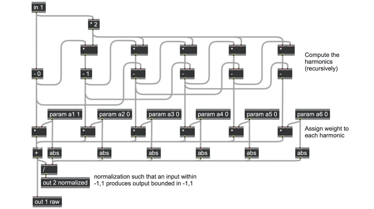
The bipolar_waveshaping_chebyshev.maxpat patch shows a few examples of computing the weights, including using exponential scaling for bandlimited impulse generation, and random walks for evolving additive drones.
Sigmoids
Sigmoids are an extremely useful class of functions that can smoothly convert a potentially infinite-ranged input into a limited range output. Here is a classic sigmoid function, the hyperbolic tangent (in gen~, this is simply the tanh operator).
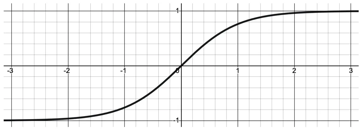
When the input is near zero, the output is near zero too, and the slope is exactly 1.0. That means, when the input is very quiet, the output signal is almost unchanged. As the input amplitude increases, whether positively or negatively, the output slope gradually tapers off, such that it curves toward but never quite reaches the limits of +1.0 or -1.0. That means that the louder the input, the more pronounced the effect of the shaping.
This makes sigmoids useful in many scenarios.[31] For example, they can be an excellent way to gain control over potentially unruly signals (not just audio!), such as might be produced by unpredictable feedback circuits. Unlike a hard limiting operation such as a clip -1 1 operator, there is no sudden point at which the waveform is cut off; instead, the limiting is softly and gradually introduced. And as it does so, it can gradually add pleasant harmonic distortion and higher harmonics.
This harmonic distortion can be quite desirable and can be intensified simply by pre-amplifying a signal before it enters the waveshaper. For example, here is a simple tanh sigmoid shaper applied to a regular sine wave, with pre-amplification settings of 1x, 2x, and 8x respectively.
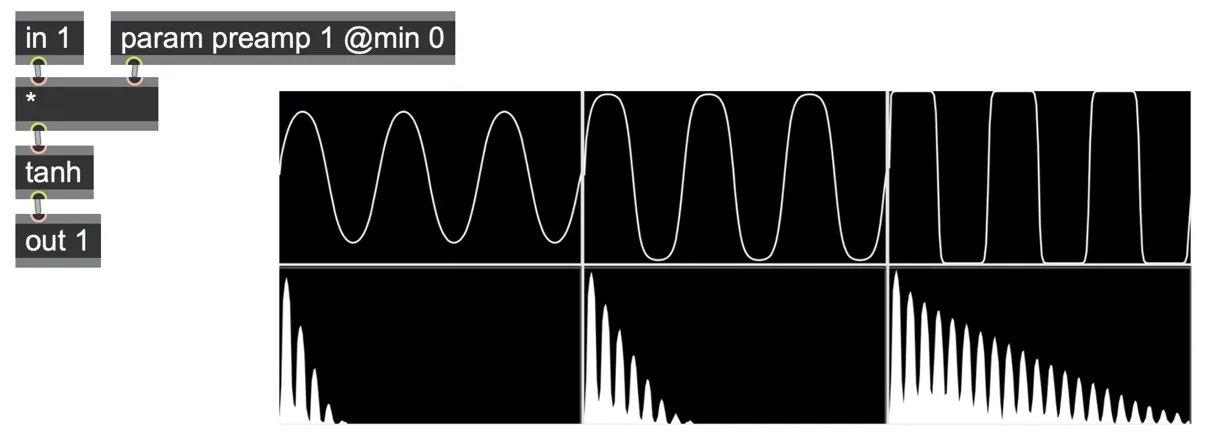
Looking at the waveforms, you can see how increasing the pre-amplification drives the sine shape toward the limits, where it approaches a square wave. The spectra underneath also show how overdriving the input increases the intensity of the higher harmonics. You can push the amplification as high as you want, and the output will never go beyond the -1.0 to +1.0 range; but it may run the risk of creating aliasing high frequencies.
The tanh operator isn’t the only sigmoid shape. Here are a few classic sigmoid shapes and their implementations, normalized to produce signals within a bipolar -1.0 to +1.0 range:
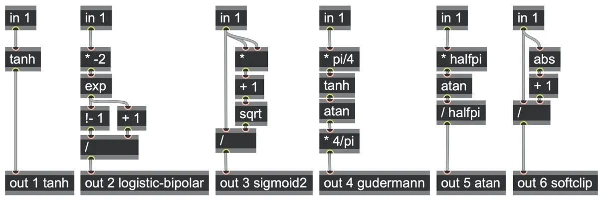
bipolar_waveshaping_sigmoids.maxpat
Each of these is also included in the book software as the go.sigmoid.tanh, go.sigmoid.logistic, go.sigmoid2, go.sigmoid.guderman, go.sigmoid.atan, and go.sigmoid.softclip abstractions.
The response shapes are very similar to each other, with the main differences being the relative distribution of energy over partials, as you can see in the spectra below.
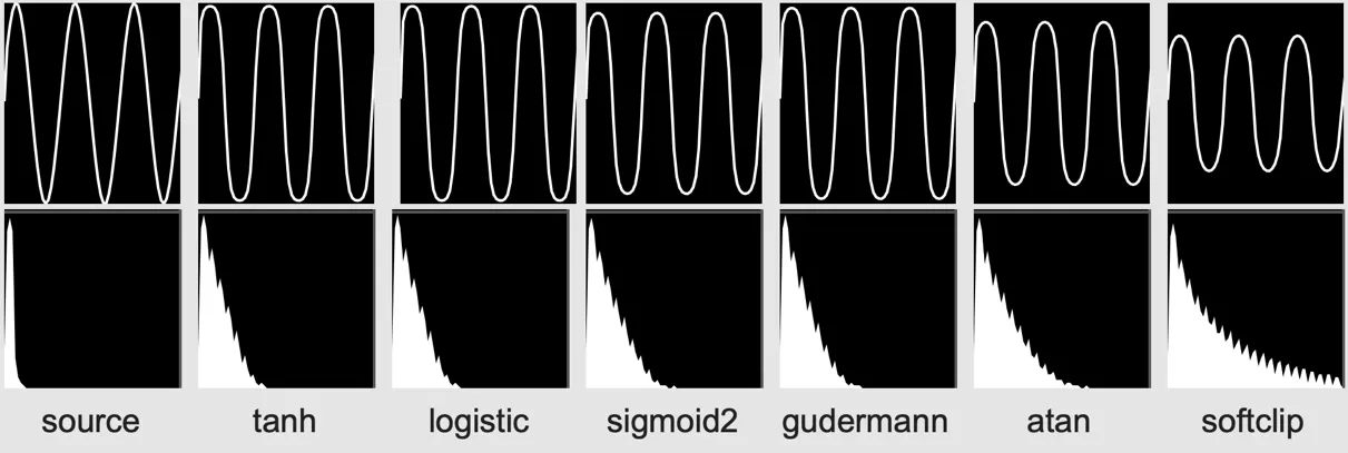
As we noted earlier in this section, waveshapers respond very naturally to enveloped sounds: as the envelope rises, not only does the sound get louder but also brighter; and as it decays, the sound also becomes duller.
The bipolar_waveshaping_sigmoids_enveloped.maxpat patch demonstrates this effect, and how the different sigmoid choices vary in spectral color to each other:
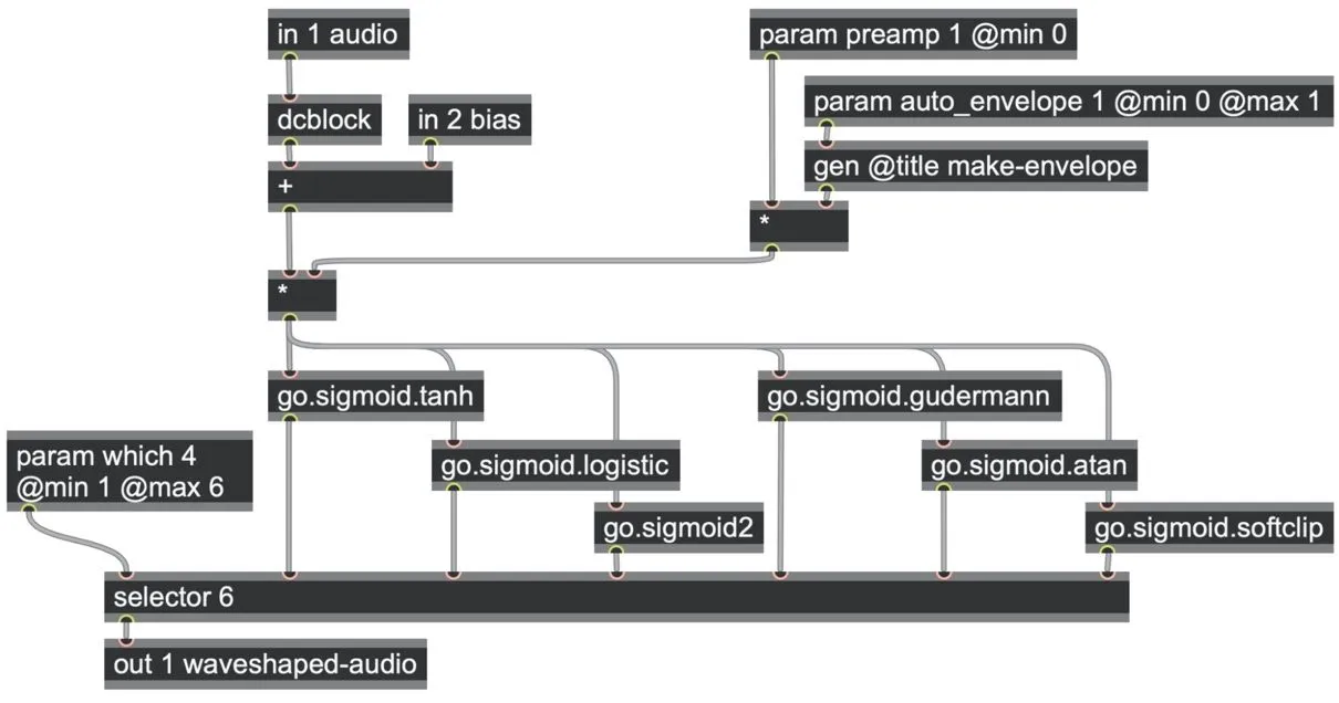
This patch also demonstrates how adding a bias offset to the Input can change the spectral response. A bias offset just means adding a constant (or very low frequency signal) that takes the average midpoint of the audio signal above or below zero. The more it moves away from the zero line, the more the waveshaping effect is different for its positive and negative halves. It may be desirable therefore to run audio through a highpass filter (such as the dcblock operator) to remove any unwanted bias, and then adding a separate input for more deliberate independent control over the bias effect, as we did in the patcher above.
Normalized sigmoids as unit shapers
Perhaps we don't always want the timbral shaping to be tied to the pre-amplification. Wouldn’t it be nice if we could modulate the curvature effect from no effect through soft shaping to extreme clipping, without making the signal quieter or louder at the same time? Then the sigmoids could also work as unit shapers.
We can easily do this by precomputing what the shaper does to the amplification factor itself, and simply dividing by that result to normalize the output. For example, if the amplification factor is x2, then a signal of amplitude 1.0 will be transformed into a signal of amplitude tanh(2), or about 0.964. Now, if we divide our shaped signal by 0.964, we ensure that the result will be a signal that once again has an amplitude of 1.0. The following patch does this, with a couple of refinements to manage the inputs.
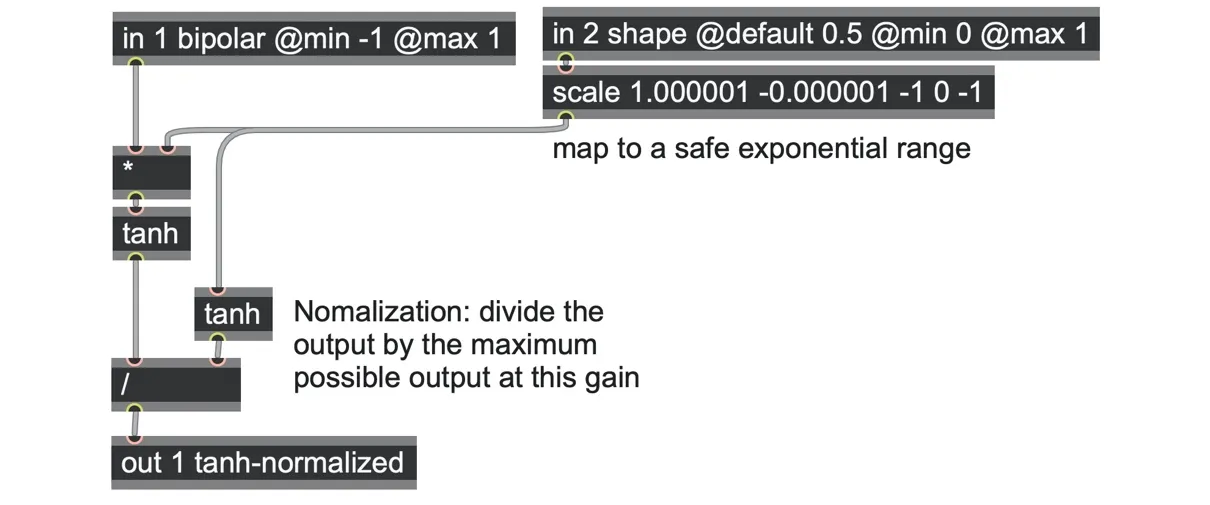
go.unit.tanh.gendsp
First, this method assumes that our input signal’s amplitude will never be greater than one, or else the division could blow up. We ensure this by clipping the input in 1 operator with @min -1 @max 1 arguments; you could insert another sigmoid shaper before this instead for less aggressive clipping.
Second, most of our unit shapers use a shape input that ranges from 0.0 to 1.0 for convenience, as it easy to swap out one unit shaper with another. To be able to generate a vast range of possible amplification factors, we take the unipolar in 2 shape input, and map it through an exponentially configured scale operator. A shape input of 0.0 produces an amplification factor of x0.000001; a shape input of 0.5 produces an amplification factor of exactly 1.0, and a shape input of 1.0 produces an amplification factor of about x1000000!
Then, to apply the normalization, we pass both the amplified signal and the amplification factor through two copies of the shaping function; and divide the results. Now when the in 2 shape is 0.0, the input signal passes through practically unchanged. And when the in 2 shape increases toward 1.0, the input signal is increasingly transformed into a maximized waveform.
The book’s software also includes unit shaper conversions of classic sigmoid shapers: the go.unit.tanh, go.unit.logistic, go.unit.sigmoid2, go.unit.gudermann, go.unit.atan, and go.unit.softclip abstractions.
Here are the results of shaping a sine wave with the go.unit.tanh abstraction at shape settings of 0.0, 0.8, and 1.0 respectively:

Feeding anything more complex than a sine wave can create some surprisingly complex output. Let's look at a perceptually interesting example of this, using a source signal that is slowly cross-fading between two different triangle waves, sent into a go.unit.softclip.
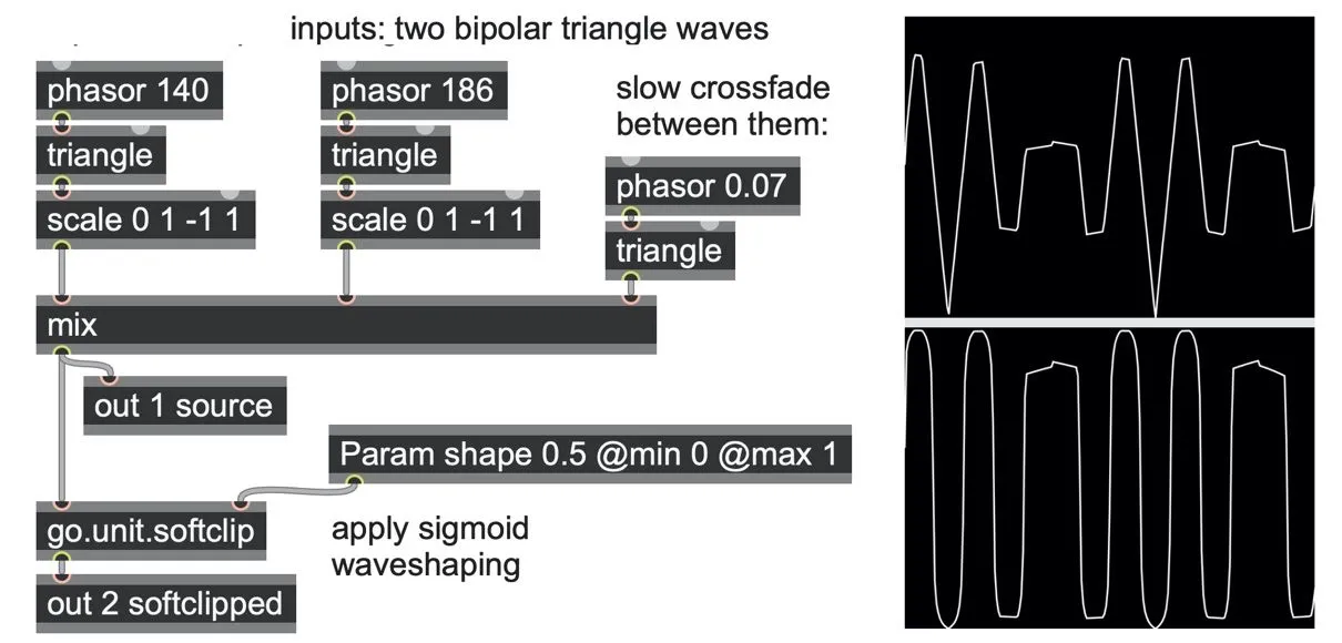
bipolar_waveshaping_intermodulaton.maxpat
The more that this input is overdriven (by increasing the param shape), the less it sounds like a crossfade and the more it sounds like a continuous pitch glide between the two tones! This kind of harmonic intermodulation between tones and amplitudes is what makes waveshaping so fascinating and rewarding for exploration.
We will return to see more kinds of waveshaping in Chapter 8, where we will see that phase modulation is just another kind of waveshaping, in which the carrier provides a periodic waveshaping function for the modulator.