Chapter 4:
Noise, Uncertainty, and Unpredictability

Throughout this book, we talk about ways that you can add variety to simple patches to achieve interesting results–moving beyond simple counting-based processes to generate and organize variety–with ideas that you can apply just about anywhere. In this chapter, we’re going to focus on the use of stochastic and unpredictable processes of noise, chance, and chaos.

The idea that the application of unpredictable processes can result in musical outcomes has been with us for a long time.[32] The list is long and interesting and includes examples as diverse as Guido D’Arezzo’s 11th-century algorithms that mapped the vowels in a text to notes on a staff, the use of isorhythms in 13th-century motets, 15th-century Netherlandic canons, Mozart’s dice games for writing minuets, Gottfried Michael Koenig’s PROJECT 1, John Cage’s use of the I Ching to generate his Music of Changes, and Iannis Xenakis’ stochastic processes.

Feel the noise

The noise operator is the primary starting point for unpredictable variety in gen~. With each passing sample frame of time, it produces a new random value in the range of -1.0 to 1.0, in which each possible value in this range is just as likely as any other, and overall the values are distributed evenly over different time scales, which means that there is no periodic pattern.

(Note that we use the term “random” here for legibility, but we should point out that, as with most computational systems, these aren’t truly random numbers, but are an algorithmically generated sequence of values that are evenly distributed, which means any value is roughly as likely to appear as any other. The sequence is so complex as to have no discernible pattern, making it practically quite unpredictable.)[33]

An audio-rate sequence of evenly distributed values with no discernible pattern sounds like a bright and rather harsh stream of noise. If it did have a discernible pattern, it would start to sound like a periodic tone or loop instead. Here is a challenge to try: how long does a loop of pre-recorded noise have to be before you can’t hear it looping anymore? You can try this out by opening the random_when_does_noise_get_forgotten.maxpat from the book’s example patches. It might surprise you.

Audio-rate noise is sometimes described in terms of colors. Just as white light contains all colors and can be filtered to produce specific hues, white noise, such as the noise operator generates, has equal energy at all frequencies but can be filtered to produce different colors of noise. (We’ll look at some filters you can use in Chapter 6.) For the most part, "color" here refers to the spectral profile of the noise, which means how much energy is distributed between lower and higher frequencies. This is perhaps a slightly odd descriptor, given that random noise is not periodic by definition! At best, perhaps we can say the noise is more or less similar to a periodic signal with high or low energy at certain frequencies.

Noise isn't just for audible timbres, but can also be the basis of random signals to control other processes. That is, the simplicity of the noise operator has a complex idea at its heart - the connection between noise (in the acoustic and psychoacoustic senses) and randomness (in more mathematical or musical senses). We’ll see this used extensively in subsequent chapters, including using random (or stochastic) output sampled at different time scales to generate melodies, spawn microsonic grains, and so on, but in this chapter, we’ll look at some more fundamental ways to use the noise operator and other algorithms to generate a variety of unpredictable signals.

Random ranges

The noise operator’s range is normalized bipolar, which simply means that the numbers are between -1.0 and 1.0. This is appropriate when we want an audio-rate white noise signal, as it covers the normal range of audio values. But if we want to use noise to drive some other random processes, we often want to scale the numbers to a different range. We can map a raw noise operator’s -1.0 to 1.0 output to any desired range between A and B using a scale -1 1 A B operator.

For example, we often want to map the noise operator’s output to a normalized unipolar range (0.0 to 1.0), as used widely throughout this book, and we could use a scale -1 1 0 1 operator for this. An even quicker way to get a unipolar output is to pass the noise operator through an abs operator. This will fold all the negative values around zero into the positive range (also known as full wave rectification).

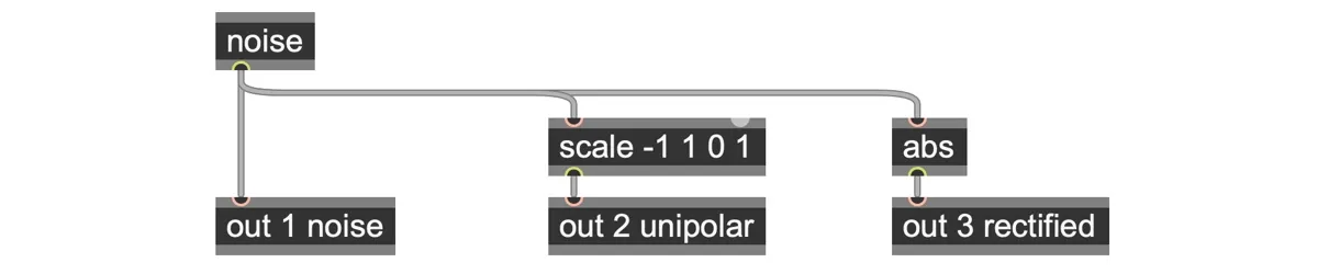
random_range.maxpat

Rate control / stepped random

The noise operator generates a new random value for every passing sample frame moment. For audio-rate noise, this is probably what we want, but for doing more algorithmic processes, we often want to control when a new random value is used. Perhaps we want a new random value on every beat, on every cycle of an oscillator, or on every note event. In this case, we can use a latch operator to “sample” noise according to a trigger (just like a traditional hardware Sample & Hold module).

In the following patch, we drive the latch by a phasor whose rate we can set by frequency using a param operator. The go.ramp2trig abstraction we built in Chapter 2 will generate triggers whenever the phasor ramp cycles.

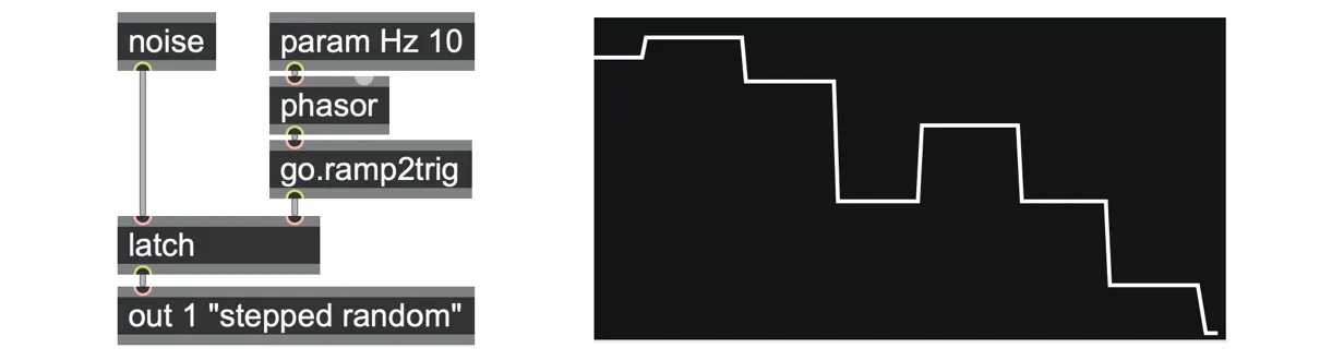
random_steps.maxpat

Once you understand this oft-used circuit, there are a number of simple variations of it that can be really useful.

Smooth stepped random

Sometimes we want a random source but without the hard edges of a raw stepped or latched random generator. We could achieve this by applying an appropriate lowpass filter or by using a slew limiter (as we explore in Chapter 6). but here we are going to adapt the "smooth-stepped" method we saw in the last chapter. In that section. rather than immediately jumping to a new random point, we used the mix operator to create a linear ramp to that point (or some other more curved, shaped interpolation between a series of random points). This time, instead of using a mix operator we’re going to do it using the interp operator.

In its default mode, the interp operator behaves effectively the same as the mix operator, except that the inlets are in a different order (the control inlet is first rather than last). What makes the interp operator more interesting for us is that it can use other interpolation functions, including multi-point interpolations, just by changing the @mode attribute. These include: @mode linear (the same as the mix operator), @mode cosine (a sinusoidal curve), @mode cubic (4-point interpolation), @mode spline (a 4-point Bézier spline), and @mode spline6 (a 6-point Bézier spline).[34]

The first inlet sets the interpolation factor, sometimes called alpha. This alpha inlet expects a value in the range of 0.0 to 1.0, which sets the amount of blending between one data point and another. Each additional inlet sets the individual data points to be interpolated between. Linear and cosine interpolations require two points; cubic and spline need four points, and spline6 needs six.

Let’s start with linear. For the interpolation factor alpha, we can simply use the phasor that is driving the go.ramp2trig. For the two points, we need both the most recently latched random value and the one previous to it. That is because the line needs to rise from the previous latched value (when alpha = 0.0) up to the new latched value (when alpha = 1.0). We can store the previous latched value by adding another latch and a history between them, like this:

This circuit is called a (two-stage) shift register. Rather like a bucket brigade, the incoming value is passed from one storage (the latch) to the next whenever a new trigger comes in. We’ll see shift registers in more detail with generative sequencers in Chapter 5.

The following image shows that happens when we put this all together:

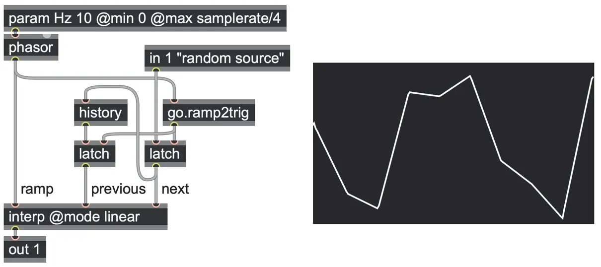
random_smoothed.maxpat

Compare this with using interp @mode spline6, which needs six input points, and therefore a six-stage shift register.

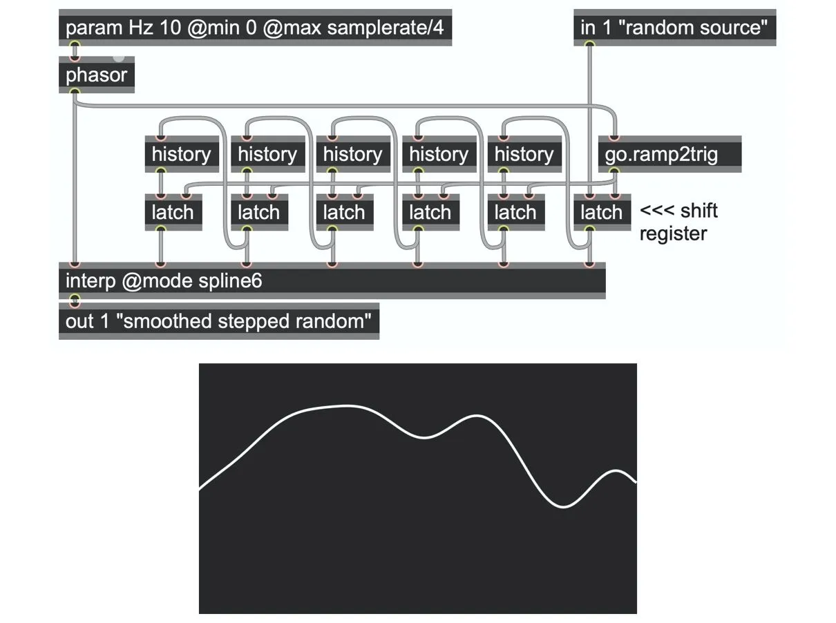
random_smoothed.maxpat (and see also go.shift.spline6.gendsp)

This technique adapts perfectly to changes in the driving phasor frequency (so long as the frequency is not negative). Each Interpolator implies a different kind of smoothing, and at audio rates this becomes a kind of sonic filtering. The random_smoothed.maxpat also shows a sinc interpolated implementation, based on an algorithm we will encounter in Chapter 9.

This general method of interpolation over a shift register works for any periodically sampled signal, not just noise. A binary chance signal, a quantized random signal, or any source—from LFOs to pitch sequences—can be smoothed in this way.

Chance and conditions of probability

Sometimes you want things to happen some of the time, but not all the time. You can create a patch that lets you create probabilistic logic signals of either 1.0 (meaning true/high/on) or 0.0 (meaning false/low/off) from unipolar noise with the addition of a less-than (<) operator.

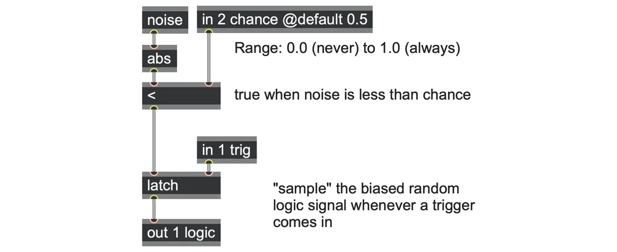
This is one of those endlessly reusable circuits which we have added to the book collection as “go.chance.gendsp”. In this case, the chance input sets the probability that the next output will be a 1.0 (true). For example, if the chance input is set to a value of 0.25, it will output 1.0 just 25% of the time and a value of 0.0 the remaining 75% of the time. Do you want to flip a coin?

Set the chance parameter to 0.5. As before, we can use the phasor-driven latch operator to control how often this decision is made.

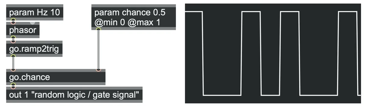
random_chance.maxpat

So now you can create a biased random decision at any moment you might need it. What you do with this is up to you—we use it in many parts of this book, and we will see it again later in this chapter.

If the chance operation is run at full audio rate, and the probability ratio is set quite low (try 0.001, for example), the result is a kind of randomized sequence of clicks or pops. Try multiplying this by another noise operator to generate dust and scratches!

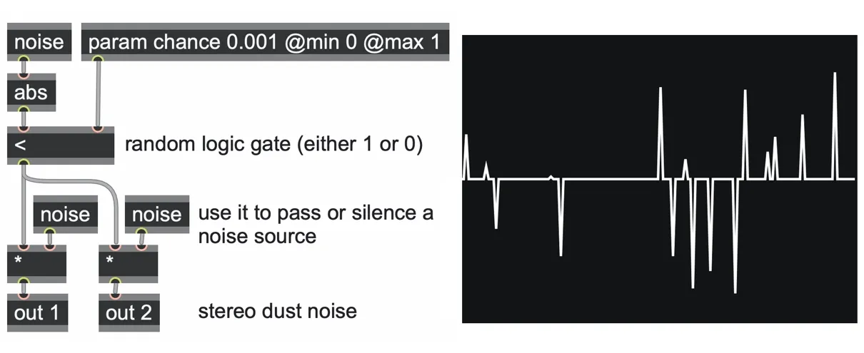
random_chance.maxpat

Bernoulli gate

A Bernoulli gate takes a trigger input and, whenever that trigger goes high, routes it to either one or another of two outputs according to some probability parameter. It can be used to skip events selectively in a series, route trigger events to two different sound sources (such as an open or closed high hat), or more generally, route event control to different sections of a patch.

Here we simply take our “go.chance” circuit from above and use the output to select between one of two outputs through a gate 2 operator. The signal input that the gate routes is the same trigger in that was used to latch the chance circuit.

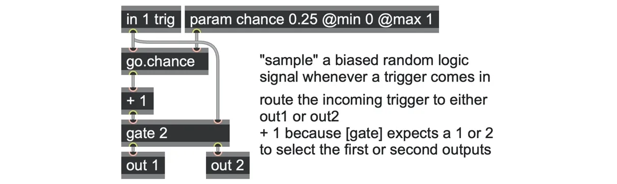
Random_bernoulli-gate.maxpat (and also go.bern.gendsp)

Random periods

Another way to generate sporadic events from a phasor-driven latch is to feed back the random sampling into the phasor’s own frequency. Every time the phasor operator ramp completes, a new frequency is sampled and held for the duration of the next phasor ramp.

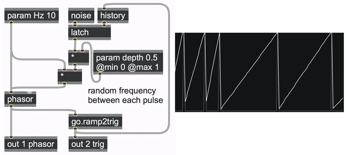
random_periods.maxpat

Here we use a latch operator to sample a bipolar noise (-1.0 to 1.0) output whenever the phasor wraps. We scale this range down by a param depth, then scale it up to the range of the param Hz to get our randomized frequency deviation. Both this computed deviation and the original param Hz signal are patched into the phasor operator's frequency input, which effectively adds them together. So, if the param depth is zero, this will output a steady phasor at 10Hz; if the depth is 0.1, it might vary between 9Hz and 11Hz; if the depth is 1.0, it could vary between 0Hz and 20Hz.

A classic application of random periods in modular synthesis is a “Krell patch”, which at its core is a sequence of enveloped sounds, where at the start of each envelope the patch selects not only a random duration, but also a random pitch and other parameters of the next sound. To do this we could take our random ramps and shape them into envelopes using unit shapers, and synchronize other latched random processes to the same go.ramp2trig.

Random distributions

The distribution of a random source describes how likely each particular possible outcome is relative to another. For the noise operator’s white noise output, all values are equally likely, so the distribution is called flat or even. We can make this distribution uneven or biased by applying different functions or curvatures to the output of the noise operator.

For example, if we feed the noise through an abs operator to make it unipolar, we can then feed that through any of our go.unit shapers from the last chapter to create a new distribution. Or more simply, if we multiply the noise by itself, which is to say, raise it to a power of 2, it will bias the distribution toward numbers closer to zero. (For example, 0.5 * 0.5 = 0.25, and 0.1 * 0.1 = 0.01; which is to say, the tendency of a power-of-two distribution on values between 0.0 and 1.0 is to make them smaller.)

One of the most important distributions in probability and statistics is (perhaps confusingly) called the “normal” distribution, and also the “Gaussian” or “Gauss-Laplace” distribution. It is one of the most widely measured distributions observed in the sciences, including for example quantum harmonic oscillators, the scales of living tissues, educational testing scores, and so on.

The simplest method of approximating a Gaussian distribution is to take an average of several random samples, but this isn’t very accurate. A much better approximation for likely similar CPU cost can be achieved using a variant of a spatial method called Box-Muller. This method generates random points in a polar 2D space with a log radial distance and returns the Cartesian X and Y coordinates as the outputs (so it actually generates a random pair of values). Both X and Y have very good normal distributions.

Here are the mathematical formulae we need:

R = sqrt(-1/4 * log(abs(noise())))
A = pi * noise()
X = R * sin(A)
Y = R * cos(A)

The last two lines of this are actually a regular polar-to-Cartesian conversion, which is available in gen~ as the poltocar operator, and we can patch up the rest using simple math operators. Since this is a really reusable circuit, we saved it in the book collection as the abstraction go.noise.normal.gendsp.

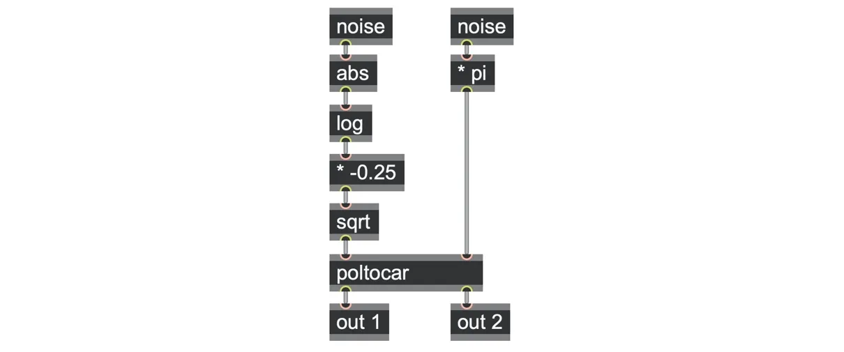
go.noise.normal.gendsp

You might have been tempted to think that changing a random distribution would also change the timbral spectrum or color of a noise algorithm. A good way to test this, and understand different distributions, is to plot them as a histogram. A histogram is simply a graph that shows how frequent (or likely) each possible output value is. The next patch shows histograms of even, exponential, and normal distributions we have encountered so far, along with a custom distribution through a go.unit.arc unit shaper.

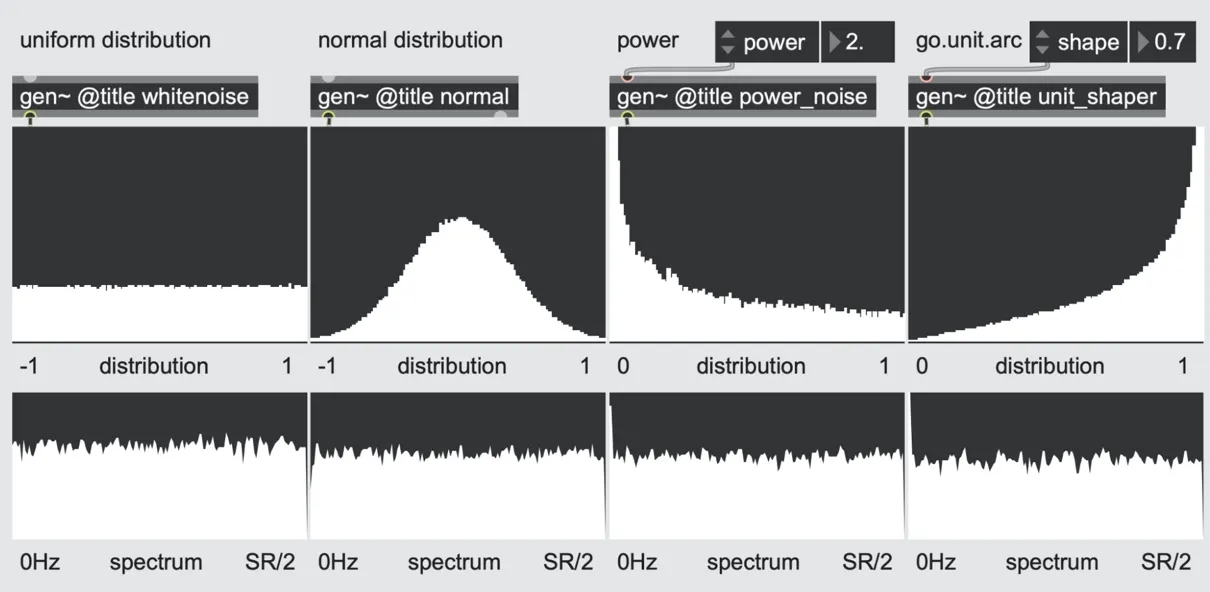
random_distributions.maxpat

As you can see in these graphs, although their distributions are all very different, their frequency spectra are all almost the same. That is, the distribution (variations in amplitude) and the color (similarities over time) of noise can be quite independent of each other.

Random walks in nature

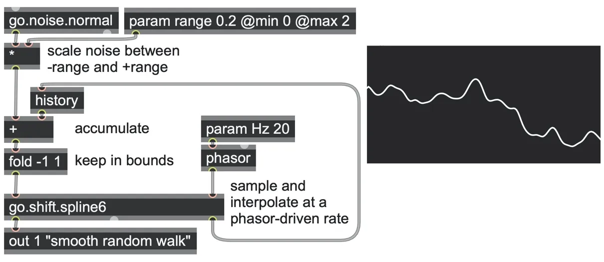
Random walks are one of the most tried and tested methods of territory exploration found in natural systems (and they also occur in simpler physical systems such as Brownian motion). The method is simply put: at each step, turn a small randomly determined amount right or left, then move forward. Each forward movement is an accumulation or integration of position: take the current position, add the random deviation, and let that be the new position.

This is similar to the drunk object in Max or RNBO. The random walk (or drunkard’s walk, as it is sometimes called) provides an interesting way to generate random outputs whose range is constrained with respect to the previous random value. That is, at each step, the output moves up or down a small, randomized amount. It is a form of counting (or integration) in which we count by random steps.

We can build a similar circuit in gen~, again using a latch to slow the process down to a desired step rate. Here the output of the latch is fed back through a history to add a new random value to it as the accumulator.

The random value is bipolar (so you can go up or down) but scaled down to some smaller range so that each step taken is relatively smaller.

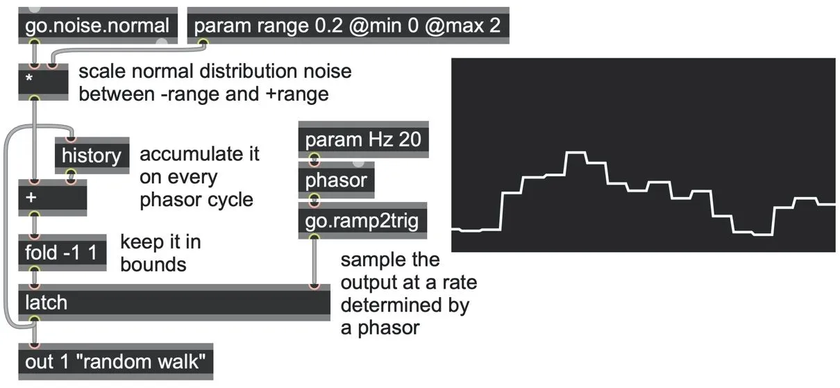
random_walks.maxpat

In the patch above, we also inserted a fold -1 1 operator into this feedback loop to stop the accumulated value from getting too small or large.[35] We also used a normal distribution of noise rather than the raw noise operator, which provides a slightly more natural random walk as it is biased toward making more smaller steps and fewer larger steps.

This patch can also run at very high frequency rates. Try running it at 10,000Hz and listen to the output while playing with the range parameter. It sounds similar to a lowpass filter: the smaller the range parameter gets, the more filtered the noise output. As we explore in Chapter 7, there is a close relationship between the sizes of waveform steps (or steepness of their slopes) and the effects of lowpass filtering. A random walk circuit pairs well with interpolated smoothing for a very natural-sounding modulation source.

Random integers / quantized random

The noise operator generates values that can be any decimal value between -1.0 and 1.0. The go.chance circuit above quantized these values into either one or zero. We can also perform other kinds of quantization to limit the output to specific values.

For example, if you only want random whole numbers of 0, 1, 2, or 3, you can scale the raw noise to a 0.0 through 4.0 range (by sending through an abs and then a * 4 operator) and then apply a floor operator to round down to the nearest whole number. Or, if you only want values of 0, ¼, ½, or ¾, you can then divide the floored integer by four again. More generally, you can quantize unipolar noise to any choice of N subdivisions using a trio of operators to handle the quantization: * N > floor > / N.

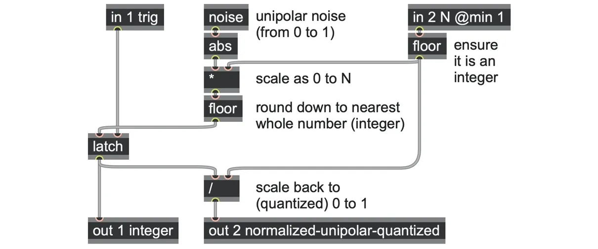
go.random.gendsp

We saw this multiply, floor, divide trio in Chapter 2 building the go.ramp2steps abstraction, and we’ll see it again in Chapter 5 for pitch quantization purposes. Here is an example using go.random to generate dice rolls ten times per second:

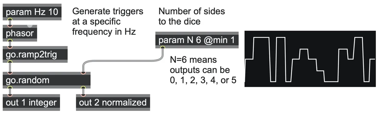
random_integer.maxpat

The urn model: pick a card, any card...

Let’s continue with random integers by diving into a slightly more complicated algorithm that builds upon a few of the techniques we have found so far.

An interesting way to select random outputs from a finite set of possibilities uses what probability theorists call the Pólya urn model[36], where each iteration of the algorithm chooses a value that cannot be selected again until all options have been used once (at which point the process begins again). For our purposes, the “urned” output could be used for any kind of table lookup, pitch computation, rhythm subdivision, sample slice selection, etc.

Why is the urn model interesting? Well, for one thing, it ensures that every item is picked the same number of times, enforcing a fully even distribution even over short periods (whereas a random number generator with statistically even distribution in the long term might not be so even over short durations). As a musical reference, this was at least part of the inspiration for the twelve-tone technique of serialist composers a century ago: if all twelve notes of the chromatic scale are sounded as often as one another, they will prevent the emphasis of any one note, key, or other harmonic bias in particular, thus liberating composers from existing tonal traditions.

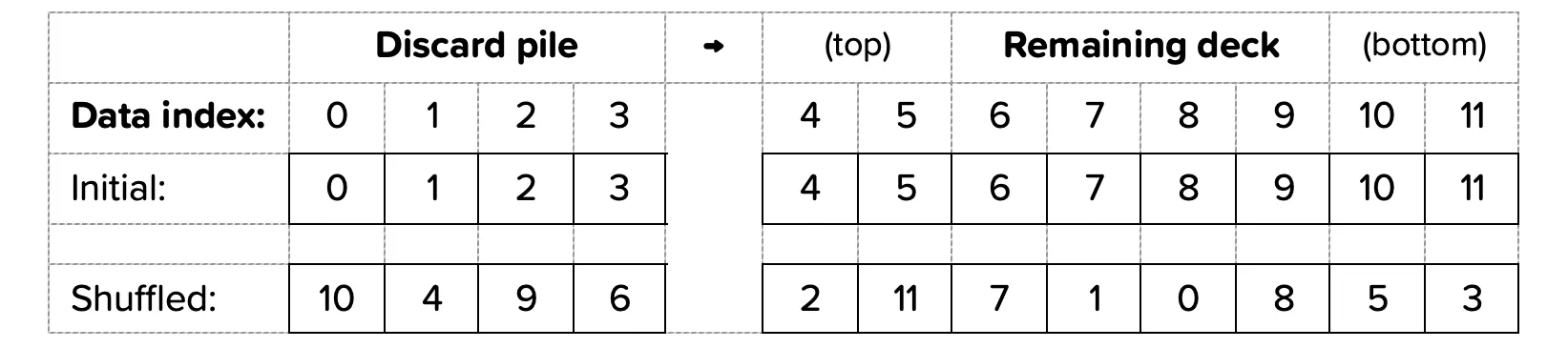
It is also one of the core methods of distributing events in many board and card games: “shuffle the pack.” Let’s imagine a deck of twelve cards, numbered 0 through 11, as a way to select pitches. The method is then a loop: The note we play is determined by the top card, which then goes on the discard pile. Once we have gone through all the cards, the discard pile becomes the new deck. The same pattern of numbers will repeat every time, creating a twelve-card (twelve-note) loop.

The urn method makes just one simple change: instead of always picking the top card on the deck, we randomly pick a card (any card) from somewhere in the deck. Everything else remains the same. Still, we play the note for that card and put it on the discard pile as before, and once the deck runs out, we simply turn over the discard pile as the new deck. The result is that, instead of repeating the same sequence every time, the sequence now has a random order each time, but each card still only comes up once.[37]

To construct this in gen~, we’ll need to store the state of the deck (and discard pile), for which we can use a data operator. For a deck of twelve cards, we can use data deck 12. Each one of the twelve slots in this data deck operator should hold one card value: 0, 1, 2, 3, 4, 5, 6, 7, 8, 9, 10, or 11.

In the midst of a game, it could be laid out something like this:

We need this deck to be set up when the patch loads, and we’re going to use a codebox operator in this case since we’ll need to do some procedural coding involving an if condition and a for loop.

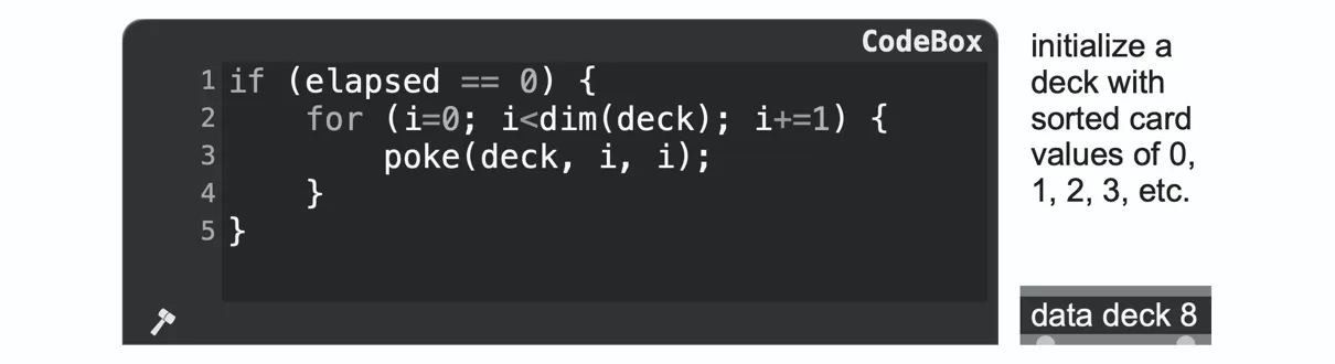
First, we want this to happen only once when the patch loads. Here we use a trick using the elapsed global variable, which always carries the number of sample frames of time that have elapsed since a patch loads. At the very first moment a patch is loaded, this value is zero. Then, on the next sample frame, it is one, and so on. Therefore, when using if (elapsed == 0) { … }, any code between the { and the } will only run once when a patch is loaded. (Incidentally, like all global variables, elapsed is also available outside of a codebox as an elapsed operator.)

When this happens, we want to update each slot of the data deck immediately. Here we use a for loop to iterate over each slot in turn and run the same piece of code for each one of them. The for loop has a loop counter variable called i, which starts at 0 (i=0), continues while it is less than the deck length (i<dim(deck)), and increases by 1 for each iteration (i+=1).

On each iteration of this loop, i steps from 0, 1, 2, 3, and so on to the last iteration, where i equals 7. Each time, we use the poke operator to write a new value into the deck. In this case, we write the value i into the slot at position i, using poke(deck, i, i). And with that, our deck is initialized!

Note also that we used dim(deck) rather than simply “hard-coding” 8 here. That way, if we decide to change the size of the data deck at a later point, we don’t need to rewrite this code.

Next, we want to step through this deck card by card. Drawing a new card would depend on receiving some kind of trigger. Here we can use a go.zerox abstraction to turn any rising-edge input signal into a single-sample impulse trigger.[38] If we feed this into a counter, where the counter’s limit is set by the size of the deck, we will get an output step signal cycling through 0, 1, 2, etc., up to 7 and then looping back to 0 with each incoming impulse. This might be a useful signal outside of the current patch, so we route it to an out 2.

To quickly test whether everything we have done so far is working (a good habit to have!), we could hook up a peek deck operator to the step value and verify that it outputs the sequence 0, 1, 2, etc.

The current step value tells us how many cards we have gone through in the deck, which is the same as how many cards are on the discard pile (and is the position of the black column in the diagram a couple of pages ago). But we also want to know how many still remain in the deck, which is just the current step (discard pile size) subtracted from the total number of cards.

We can now choose a random integer with the range of what remains using the same noise, abs, multiply (*), and floor method we saw earlier and adding (+) this to the current step to get a random index within the remaining deck.

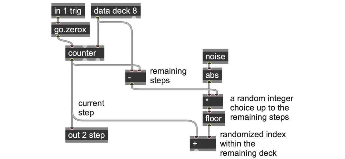
Now we have two indices into the data: the index of the current step (the current card) and the index to swap it with (a randomly chosen card in the remaining deck).

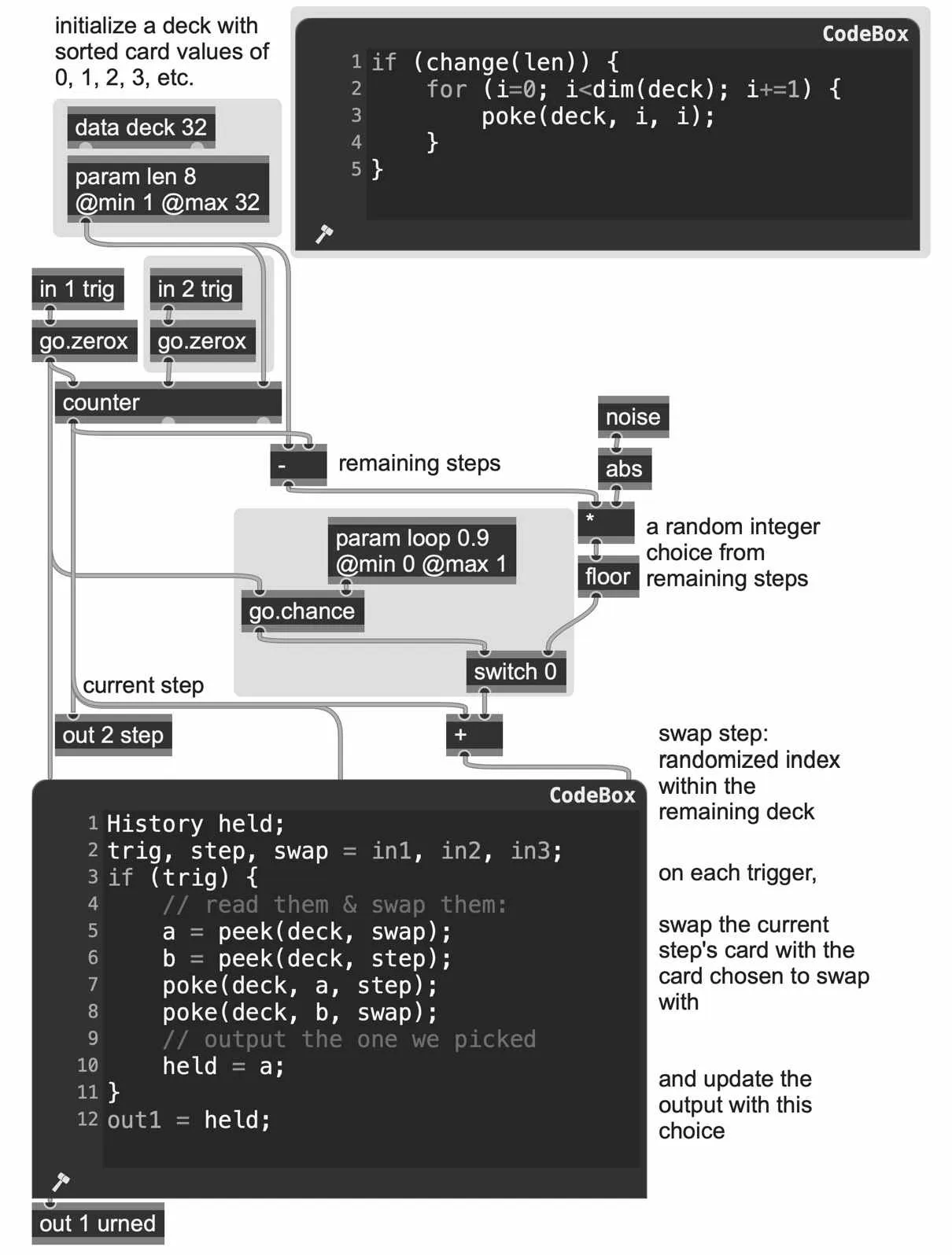
The swap should only happen when the clock ticks, not on every sample frame of passing time. That is, when a trigger is received, we draw a new card from the random location of the deck and hold that value until the next trigger. With visual patching here, we’d probably reach for a latch here, but since the swap will involve several operations, using a simple latch isn’t ideal. Instead, we will turn to a codebox again to use an if block to control when a series of operations can take place (in this case, selecting and swapping a new card). We would like this card value to be remembered and continually output between each trigger, and anything remembered needs to be written into a history.

Let’s start with the framework of code we’ll need for this and look through each part in turn:

History held;

trig, step, swap = in1, in2, in3;

if (trig) {
// things here happen only when in1 is nonzero
// if in1 is a trig impulse signal, this is
// only when it “fires”
// here something will assign a new value to the “held” history
}

out1 = held;

First, in a codebox, history operators need to be declared at the top of the code before any other instructions since they are visible to all code and therefore must exist before any code can run. Such declarations are required to be capitalized as History (which has the benefit of making them more visible). These requirements are also true when we use Param, Data, and Delay.

Next, we declare the inputs to the codebox. In general, to connect a codebox with the surrounding patch, we need to use some inputs (using in1, in2, in3, etc.) and assign some outputs (using out1 = 0; etc.). Simply mentioning in3 in the code will give us a codebox with three inlets, and assigning to out2 would give us two outlets. (Note that there is no text space between “in” and “1” here; “in1” is one word.) It’s a good habit to plan to declare these in the codebox before writing other code, just as it is a good habit in patching to create the in and out (and param etc.) operators before patching up an algorithm. In our case, we need the trigger input, and we also need to feed both the current step and swap indices into the codebox. We also need one output at the end for the currently held card.

Between the inputs and outputs, we have our if block. An if block needs a logical condition to test to determine whether its block will run (if the condition is nonzero) or not (if the condition is zero). In this case, we use the incoming trigger as the condition so that the block of code it contains only runs per each incoming trigger tick.

So now all we need to do is fill out the body of this if block. The task here is to swap the cards at the step and swap indices. That means we need to read the data (using peek) to find out what each card value is and then write these values back to the data (using poke) with the indices swapped. Notice here that using a codebox operator also ensures that our reads and writes happen in the order we need them to:

// read both positions:
a = peek(deck, swap);
b = peek(deck, step);
// write them back, swapped:
poke(deck, a, step);
poke(deck, b, swap);

And finally, it’s the card “a” at the random index that we actually chose, which the urn algorithm should output:

held = a;

Put all together:

random_urn.maxpat

Here is an example trace of the output with the step signal (gray) against the current urn output (white) which plays every card exactly once:

A more flexible urn

We can extend this patch a little further to get some very useful features.

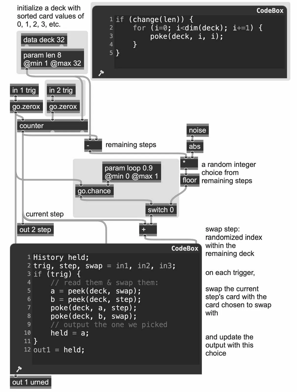
For example, we can add a second trigger input to “reset” the counter back to zero (using the counter’s 2nd inlet) so that we can synchronize the pattern with another clock.

We could also make the size of the deck be configurable as a parameter (up to some limit of the size of the data operator). That just means adding the param operator and using the parameter value instead of the data length. In that case, we probably also want to re-sort the deck when this parameter changes—which we easily can do by substituting our elapsed() == 0 condition for a change(len) condition).

More interestingly, we could choose whether to perform the urn swap or simply continue looping an existing pattern according to a param loop control. If looping is enabled, we do not need to randomize the swap position or perform the swap. We can either bypass the swap code, in this case, using another if block, or we can simply set swap to equal step to achieve the same result with simpler patching.[39] This creates a quite performable tool: disable looping for a while until you find a pattern you like, then flip looping on to keep that pattern running for a while until you feel like you want it to change again.

We could even make this choice probabilistic using our earlier go.chance circuit; we can have the algorithm loop for, say, 90% of the time and swap cards 10% of the time for a more structured but still random variety. By setting the looping probability high, the loop will evolve very slowly. If you want to scramble the pattern, set the probability to zero. We’ll encounter this kind of probabilistic evolution of a pattern again when we look at using shift registers as a way of creating sequences in Chapter 5.

Here are all of those changes made to our random_urn.maxpat patch.

Chaos (and why we like it)

Alongside stochastic sources, there’s another category of functions that are of great use as an alternative for controlled unpredictability: chaotic equations.

The equations we’re talking about when we use terms like chaos or chaotic attractors are not actually random at all. They are really a class of mathematical equations whose output over time is also quite deterministic but nevertheless unpredictable in a way that is different from the deterministic unpredictability of noise. A chaotic system’s behavior can be very sensitive to its initial conditions, falling between one set of characteristic behaviors (one “attractor" or another). It might hold steady for a while in one such regime before suddenly switching to another. Or, more simply, it might seem to oscillate in a characteristic way but which nevertheless, unlike a typical periodic LFO, does not exactly ever repeat. It’s all about sensitivity and variation.

When you think of music, it’s easy to characterize it as starting with a simple unit - a motif or a timbre - that’s transformed or distorted over time and perhaps then followed by some kind of return to the material it started with. Chaotic equations are a useful category of compositional or improvisational tools for creating such A-B-A* transitions in your work. The possibilities extend over a broad range of scales, from generating timbres at a very low level, up to phrases and on to larger formal kinds of organization. Chaos is one of the ways to ride that line between tedious repetition and incoherent randomness, which happens to be a line where the complexity, and the useful information content, increases.

A Lorenz attractor

Let's create a patch that enacts the Lorenz attractor[40] — a system of three equations used to develop a simplified model of atmospheric convection (this same set of equations also shows up in models of forward osmosis, brushless DC motors, and some chemical reactions).

Each of the three equations defines the changes of a single dimension, called the X, Y, and Z variables. Since these are equations of change, they are defined as the deltas (using the Greek letter “∂”) of each dimension. On each step of passing time, this change (delta) is accumulated (integrated) onto the dimension’s value. (So, again, this is a kind of counting!) The change is scaled by a ∂t (“delta-T”) amount to indicate the rate of passing time. The resulting changes are added to the X, Y, and Z values and then stored to be used when the next cycle of the system is calculated.

So, in a way, each of these equations models a kind of motion, much like our random walks, ramps, and other accumulation-based algorithms throughout the book. What makes this system nonlinear is that each of these changes is dependent on the previous X, Y, and Z outputs in a feedback loop, and what makes it chaotic emerges from the specific ways these feedback interdependencies cause unpredictable trends over time.

Our patch is composed of three basic sections:

1. The patching necessary to represent the calculation of the individual X, Y, and Z values.

2. The patching that stores and recalls the last iteration of the system and outputs the current X, Y, and Z results.

3. The patching that provides the representation of time used to increment the result of the current calculation.

Let’s start with the three equations in the system. Here is the Lorenz equation in its basic form. It includes three parameters (a, b, and c, set to values of 10, 28, and 2.6667, respectively).

∂x/∂t = a * (y - x)

∂y/∂t = (x * (b - z)) - y

∂z/∂t = (x * y) – (c * z)

Since these dimensions of X, Y, and Z need to persist over time, we can declare them in a patch as history operators. The initial values for each of them are set to 1.0, so we declare them as history x 1, history y 1, and history z 1.

Although the Lorenz equations are defined as continuous differentials (∂x/∂t etc.), our patches are operating in a discrete sampled time in which each step is a finite difference of one sample-frame’s duration. On each step, we compute the finite difference and scale it by some very small “dt” value. This small amount is then added and fed back to update the stored history value. As code, it could be written something like this:

x = x + dt * (a * (y - x))
y = y + dt * ((x * (b - z)) - y)
z = z + dt * ((x * y) – (c * z))

As a patch, it looks like this:

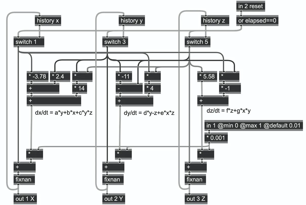
chaos_Lorenz.maxpat

The small dt we use as our time unit should be the same for all three calculations. Choosing a very small value for dt will output the results at a smooth and controllable rate, while increasing the dt value will bring the attractor code up to audible output rates, too. (But don’t expect the resulting outputs at audio rate to be “in tune” with anything but themselves!) The param dt 0.01 @min 0 @max 1 and * 0.01 operator pair sets a reasonable range for the dt values.

We start at the top with the trio history operators, whose arguments set the initial X, Y, and Z values. (Using the history operator also gives us a way to restart the calculation by sending the message reset to the gen~ object or override specific states by sending x, y, and z messages.) Those history operator values are used to calculate a single iteration of the equation. Each of these previous X, Y, and Z values then feeds into the equations for each dimension’s rate of change. These delta values are then multiplied by the dt parameter to produce smaller and more controllable increments. These dt-scaled increments are then added to the previously stored X, Y, and Z values to compute the new X, Y, and Z values, which are output from the patch and also routed back to store into the history operators for the next iteration.

The chaos_Lorenz.maxpat patch shows the attractor in action, plotting each of the three dimensions over time and visualizing each pair of dimensions as a 2D Lissajous plot (which reveals the characteristic butterfly loop shapes).

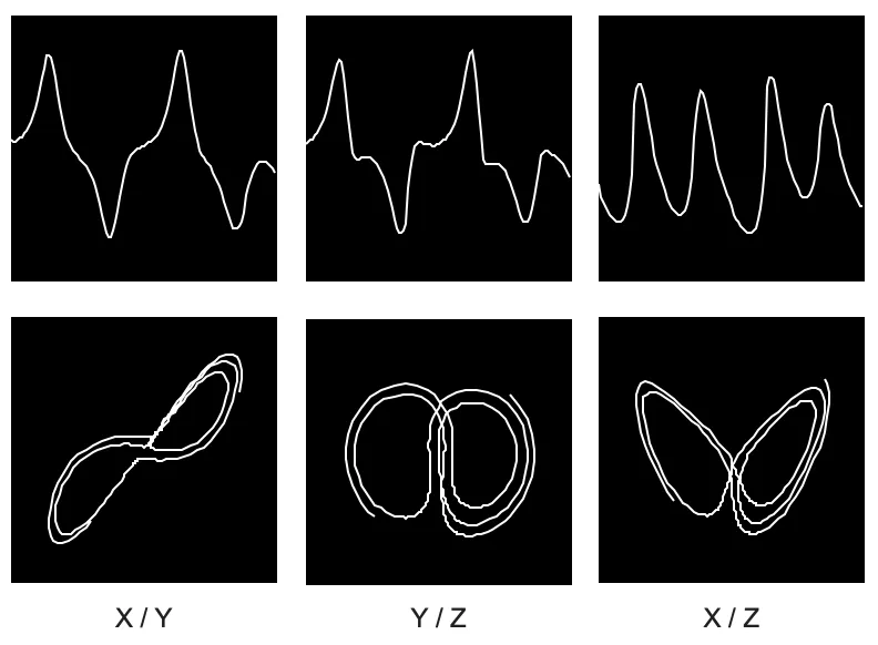
Over time, you can see some almost periodic motions (one cyclic attractor) punctuated by sudden swoops and dives into different periodic motions (another attractor). In the 2D plots, it is clearer how each cycle is slightly different to the previous one, even within a single attractor.

If you route one or more of the outputs to an audio output and increase the dt up to around 0.1, you might start to hear a low rumble. Keep going up, and you can hear a somewhat noisy, intermittent tone, or perhaps a complex of two noisy tones with sub-rhythms. (The scope view might look quite jagged, but this is just a limitation of the scope resolution.)

Finding the limits

One other little catch that we didn’t mention yet: most chaotic equations operate over quite limited ranges of values and usually will need to be rescaled (using a scale operator, for example) for most useful applications. With the Lorenz equations, the X value ranges between around -22 to +22, the Y value between around -29 and +29, and the z value between around 0 and +54. So, in our patch, you may have noticed that we scaled our outputs to a normalized bipolar range (-1 to +1) using a scale -22 22 -1 1, scale -29 29 -1 1, and a scale 0 54 -1 1, respectively.

These ranges are often not published alongside the equations themselves, but we can find them out easily enough by keeping track of the attractor’s minimum and maximum outputs over time. Here is a bit of patching to track the lowest and highest values of any incoming signal by looping min and max operators through history operators. We use a switch operator to initialize (and have the option to later reset) these minima and maxima with extreme cases, rather than zero, in order to catch signals that never swing positive or never swing negative at all.

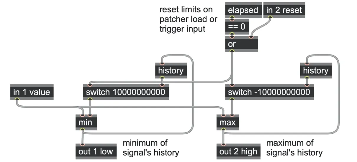
go.limits.gendsp

We can use this go.limits abstraction to find the highest and lowest values of each output of any signal’s history. Better still, we can use these values with a scale operator to keep our output within a desired range (here specified to be bipolar by param lo and param hi).

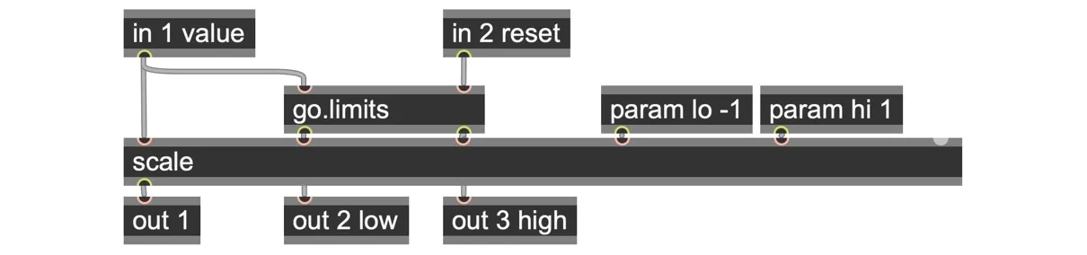
go.autolimit.gendsp

We can use this go.autolimit abstraction on each of the outputs from our Lorenz attractor equation to keep them in a normalized range.

For any specific chaotic equation, you could probably run the go.limits abstraction for a while and read off the reported low and high peak values from number~ boxes in a Max or RNBO patch, and then write those values as constants into scale objects in your patch, just as we did for our Lorenz attractor earlier.

There’s one other limit to watch out for. As you work with these chaotic attractor equations or port your own, you may notice that setting the dt parameter to larger values can sometimes make the attractor “blow up.” That can haIecause increasing the dt parameter is effectively decreasing the sampling resolution of the chaotic equation itself. This can cause bigger jumps along the function between each calculation that can lead to too much overshooting or undershooting of the curved function, as it is approximated by linear segments until it shoots off to infinity. That’s the reason that nearly all the chaotic attractor code out there explicitly mentions what the dt parameter should be and the reason that we limit the dt param from going beyond a maximum value.

go.chaos

This book comes with a collection of patches modeling other chaotic attractor equations besides the Lorenz system, which you can use in your patching. You’ll find many patches in the examples folder and also many go.chaos abstractions in the patches folder.

For example, here’s the Liu Chen attractor from go.chaos.liu_chen with go.autolimits to keep it in bounds and an extra averaged output for a bonus signal:

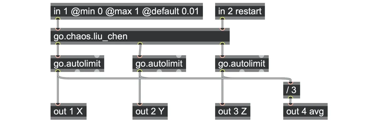
Liu-Chen.maxpat

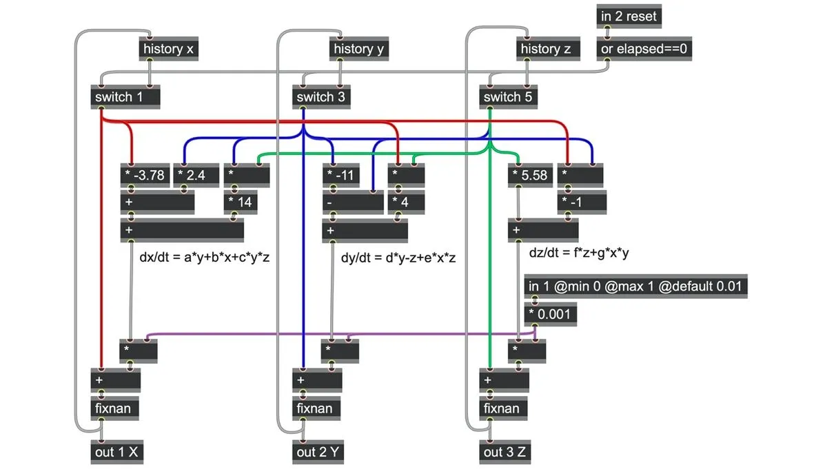
go.chaos.liu_chen.gendsp

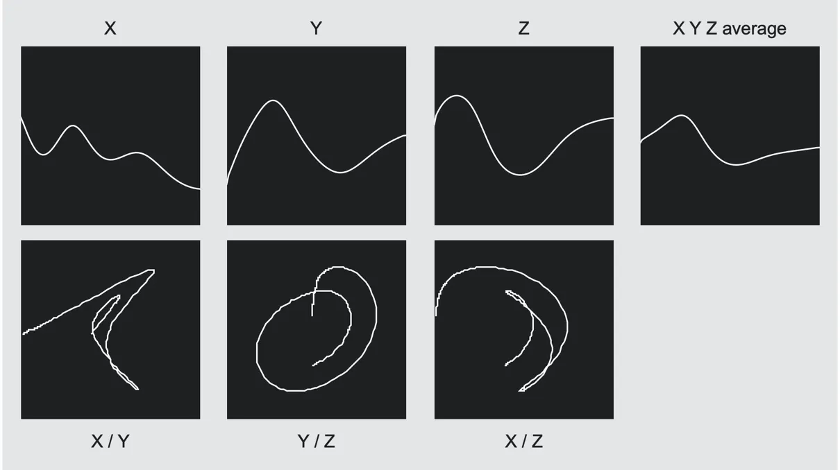
Liu-Chen.maxpat

Balancing order and unpredictability

Working with sources of noise, randomness and chaos is always a balancing act between unpredictability and control.

Unpredictable signals can sometimes seem too boisterous and take over the character of a sound, but there are many ways we can tame and gain control over them. We’ve seen how we can control the ranges, skews (distributions) and quantizations of random levels; as well as how sporadic sampling over time can reduce noise to timed chances and choices, which we can synchronize as desired. We have also seen how filtering, smoothing, and integration can soften noise and stepped into continuously wandering fluctuations (and shape the audio spectrum).

Conversely, we can use unpredictability to counteract the overabundance of control and stale repetition that digital processing offers by default. Adding a small amount of random walk, smoothed noise, or chaos to almost any parameter is a simple way bring an algorithm to life. Doing this to two copies of an algorithm can create compelling stereo space. Even mixing barely perceptible noise into audio can create a sense of natural air. Or at a slower rate, we can find evolution through occasional deviation such as the near-looping patterns of the urn model (and of the shift registers we’ll see next chapter).

But before moving on, let’s look at a couple more examples of balancing order and chaos.

Example: adding natural looseness to a tempo clock

Digital clock tempo sources are highly accurate, but sometimes this accuracy can come across as overly robotic or non-human. Aside from warping a ramp-based clock for swing as we saw in Chapter 3, we can also add micro-modulations to the ramp to reduce the robotic qualities of a rhythm through slight indeterminacies. Such deviations will also carry through to any other ramps derived from it.

A chaotic attractor is a wonderful source of unpredictable deviation that can simply be mixed into the frequency (or slope) of a tempo clock ramp to produce anything from a little variation, to loose, sloppy, or even downright wonky play.

Here we used a Coullet attractor system, autolimited and scaled by a param humanize control, to disturb the slope of a ramp-based clock:

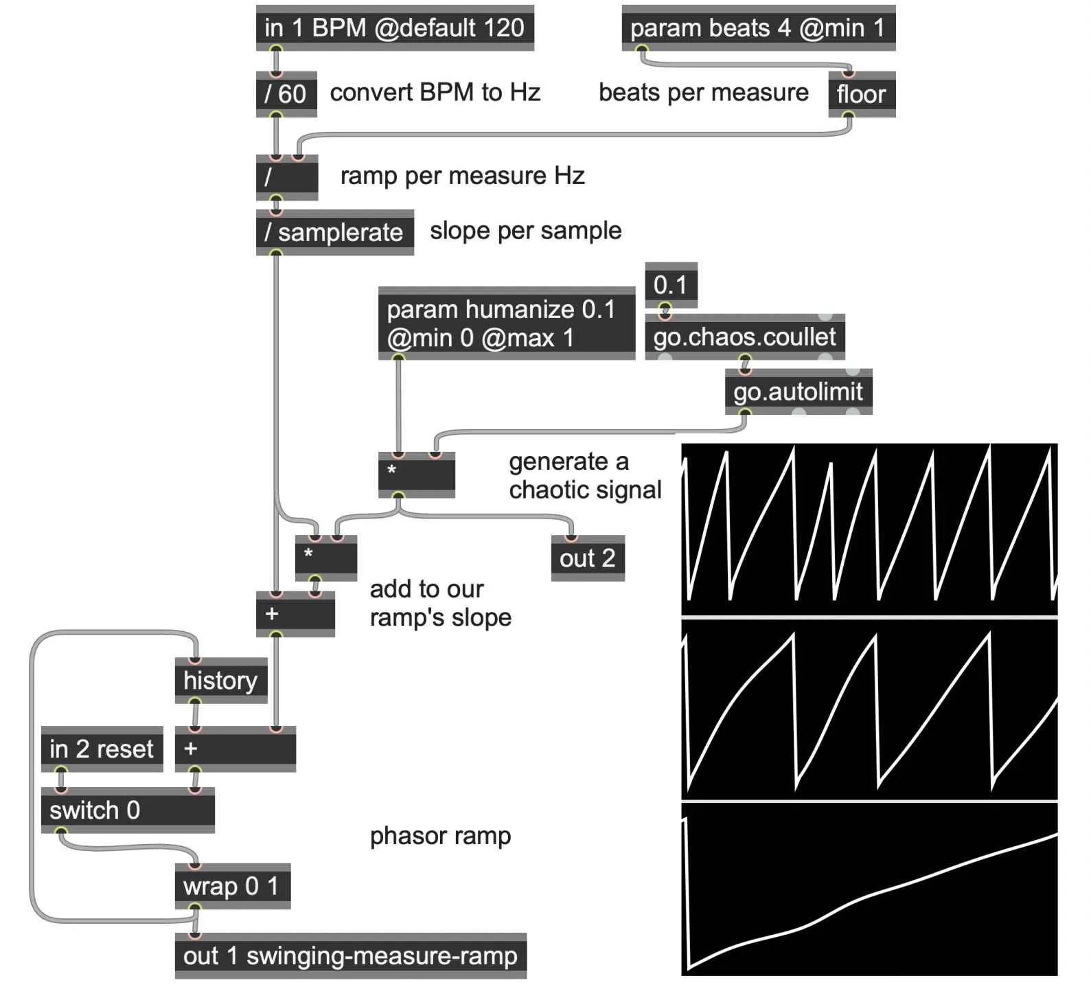
chaos.tempo.nonrobotic.maxpat

Example: injecting audio into chaos

After translating mathematical equations into patches, we can of course start to modify them to gain more control over them. For example, in this patcher, we added in operators to allow us to insert audio signals directly into the recirculating feedback loops, in order to sometimes drive the system away from its attractors.

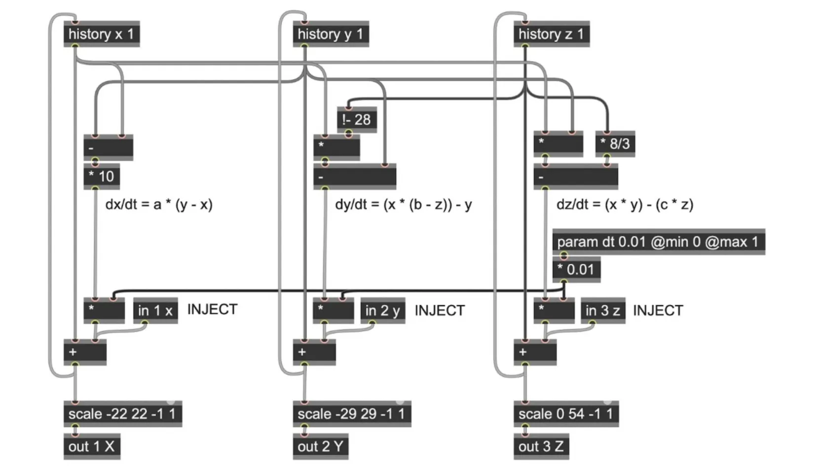
chaos_Lorenz_audioinjection.maxpat

Try mixing a sine or triangle wave into the in 2 Y input and vary the param dt to hear something like filter with noisy instabilities! The louder the input signal, the more it takes control.

Why not explore inserting other signal processes from elsewhere in this book into these feedback loops: perhaps a sigmoid waveshaper to control those blowups, or a smoothed bitcrusher to steer the attractors, perhaps a filter for extra ripple, perhaps a delay for strange harmonics. This kind of exploratory flexibility is part of what makes gen~ so valuable!