Chapter 2: Modular (Arithmetic of) Time

There are many ways to think about time. There are pasts, presents, and futures, or perhaps nested sets of shorter and more enduring moments. There are births, lifetimes, and decays, with moments imagined and forgotten. And there are repetitions and measures of time, from the natural cycles of heartbeats and seasons to the rhythms and beats of music and the oscillations and resonances of sound.

In this chapter, we’re going to look at how we keep count of time. We’ll show you how we handle both linear and cyclic time in gen~ and how widely that can be applied–for oscillators, sample players, loopers, rhythm generators, LFOs, and more. We’ll model cyclical time as a ramp whose positions along a repeating timeline can be thought of as phase and how representing musical time as a set of ramp functions provides you with more information and greater flexibility and opens up more powerful ways to modulate musical time.

Counting by sample frames (accum)

In our everyday lives, we measure time by counting intervals (minutes, hours, days, years, etc.) as well as measuring in comparison to those known rates—minutes per hour, days per week, etc. The act of counting time is also central to much of the work we do in gen~ and is a recurrent theme of this book. Like other digital signal processing (DSP) environments, the passing time of a signal is sliced into sample frames at a rate defined as the sampling frequency or samplerate: the number of sample frames that pass per second.

This rate is typically faster than we can hear (44,100 or 48,000 samples per second are common sample rates), fast enough that we can compute and generate sounds up to the highest frequencies that we can hear. Since the operators in a gen~ patch are always working, they perform their function once for every passing sample frame. In the gen~ world, each operator performs its operation in turn within a single “sample frame” so that the entire patch moves forward as a whole, one sample frame at a time.

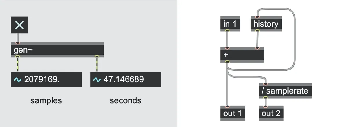
The counter_simple_timer.maxpat patch shows the simplest form of counting time by samples; we create a patch that adds one to itself on each sample frame. This needs only two operators: a + (plus) operator to do the sample-by-sample addition and a history operator to keep track of the result from one count to the next. We’ve also added some patching that lets us see how much time has elapsed.

counter_simple_timer.maxpat

In this example, we use a toggle object to enable the counting. Remember that signals are always flowing in the gen~ world. That means everything is always on unless you make it do nothing. For example, the in 1 operator in the gen~ patch above continuously outputs numbers. When the toggle object is turned on, it sends a value of 1.0, so the in 1 operator outputs a continuous stream of 1.0s. This sets things going, counting in ones. Turning the toggle off sends a zero, which sets the in 1 operator to output a continuous stream of zeroes. This appears to “pause” the counting, but really, the patch is working away—we’re just adding zeros with each tick of the sample clock, so the total doesn’t change.

You may notice that the count gets very large, very quickly. That’s because our accumulator is working at very high speed, adding one for every passing sample frame. At a typical sample rate of 44,100Hz or 48,000Hz, that means we are counting by adding one, tens of thousands of times every second.

If we want to work in other measures of time beyond the single sample frame — such as seconds or milliseconds or beats, etc. — we need to specify how many samples constitute these longer spans of time and use that value when we do our calculations. The gen~ object automatically keeps track of the sample rate currently being used by the parent patcher and provides a constant operator (samplerate) that lets us perform calculations based on this rate.[13] For example, in the patch above, we divided our sample count by the samplerate to calculate the elapsed time in seconds.

What we have made here is a timer. The output of this patch will tell you how much time (in sample frames and in seconds) elapsed while you had the toggle turned on.[14] We can also think of the count as a position along a timeline. When the output count is zero, we are at the start. As the output count increases, we are moving through the timeline. Compare this to the transport control in a sequencer or wave editor: with the toggle input, we can pause and resume playback.

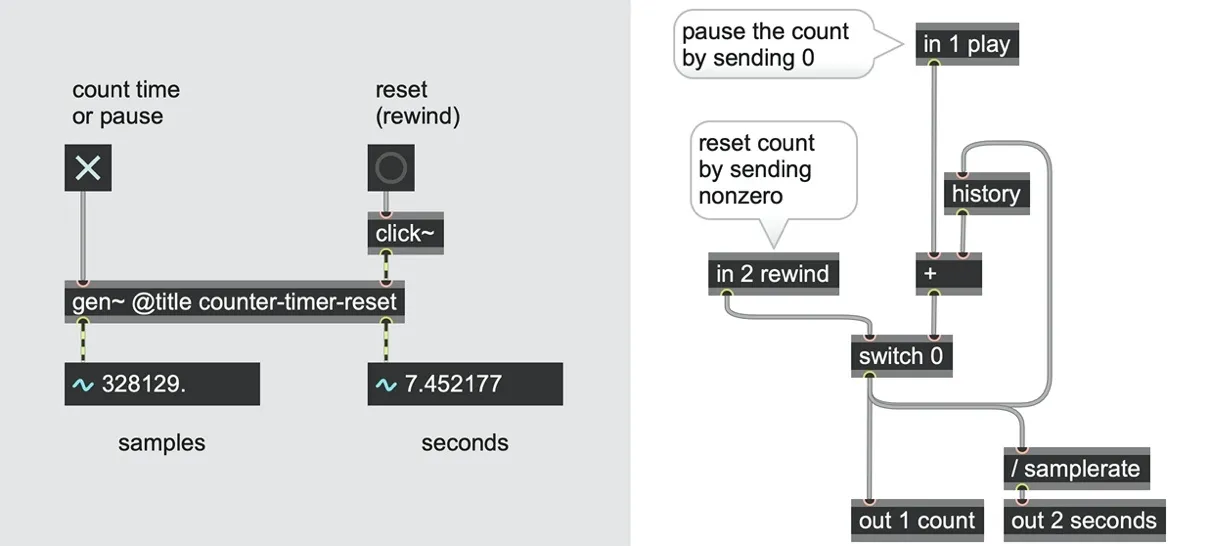
What if we want to rewind back to the start? We can add the ability to reset our accumulator by adding a switch operator and a second inlet for the reset input.

counter_timer_reset.maxpat

What does the switch 0 operator do here? If the left inlet is “false” (which means a zero value), it routes its right inlet to the output (in this case, our current count). Otherwise, if the left inlet is “true” (which means any non-zero value), it will route its middle inlet or argument (in this case, the argument 0) to the output.[15] Since this switch is now in our accumulator feedback loop, when it outputs a zero, the running count will be reset back to zero. In our parent patch, we use the click~ object to produce a single-sample trigger (a signal that has a value of 1 for a single sample frame and then returns to zero again) to perform this reset.

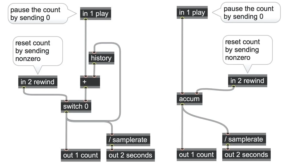
This simple patch is so useful that it exists as a built-in operator, called accum, which you’ll see in wide use throughout this book. Both of the following patches do the same thing.

counter_timer_reset.maxpat (left) and counter_accum.maxpat (right)

On every sample frame of passing time, an accum operator will keep adding up whatever you send to its left inlet and outputs the running count from its outlet. You can reset this count back to the start by sending a non-zero value to the accum operator’s right inlet.[16]

Playing a sound file

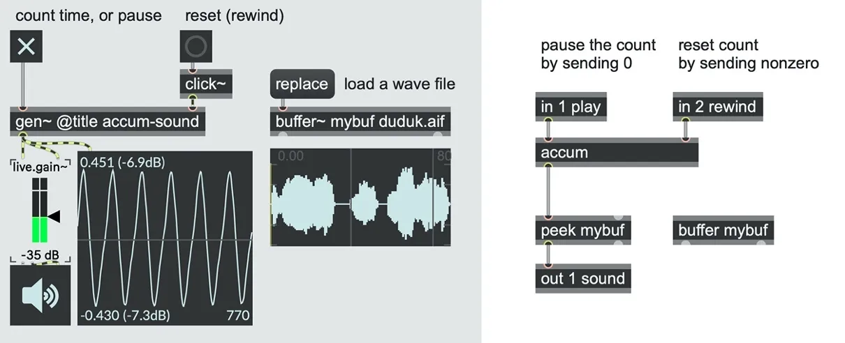
As a simple example, let’s use a count of elapsed samples to play back the content of an audio file, sample by sample.

First, we’ll need to bring a sound file into the parent patch, using the buffer~ object, with a name we can refer to it by, such as “mybuf”. If we have an audio file in Max’s search path or want to use one of Max’s built-in sound files, such as “duduk.aif”, then we can have buffer~ auto-load this file using arguments in the object box (buffer~ mybuf duduk.aif). Or we can also use the buffer~ object’s replace message to load a different audio file, and it will also automatically resize our buffer~ length.

To access this data from inside of a gen~ patch, we’ll need to add a buffer operator inside of the gen~ patch. We can link the gen~ buffer to the parent patch buffer~ by giving both the same name, e.g., buffer mybuf.[17]

Now that we’ve associated our gen~ buffer with the buffer~ object in our paren Max or RNBO patch, we need a way to read sample data out of it. The simplest way is to use the peek operator, which requires the name of the buffer to read from; in our case, peek mybuf. Since our accumulator will count every sample of audio in the buffer and do so one sample at a time, all we need for playback is to take the current sample count output from our accum operator, send it to the peek operator’s first inlet to fetch the corresponding sample value from the buffer, and then route the peek operator’s outlet to send that audio to our patch’s output.

counter_play_a_buffer.maxpat

The counter now rewinds and the wave file plays again whenever we hit the reset button. We have built the simplest retriggerable sample player.

Looping with modular arithmetic

As a timeline, the count of an accum operator goes on forever (or until you reset it). But the wave itself file is a finite number of sample values; pretty soon, the timeline has gone past the end of the wave file’s data, and there’s no more sound. What if we want to work with a looping timeline to make the sound file repeat?

We can easily turn our linear counter into a looping counter by feeding our accumulator through a wrap operator. The wrap operator lets us set low and high limits for a signal, and whenever the input goes above the higher limit, it is “wrapped” back down and starts again from the lower limit. Similarly, if we count down and cross the lower limit, our count is “wrapped” around up to the upper limit. This kind of mathematics is known as modular arithmetic.[18] We use it all the time with clocks, angles, sawtooth waveforms, and rhythms.

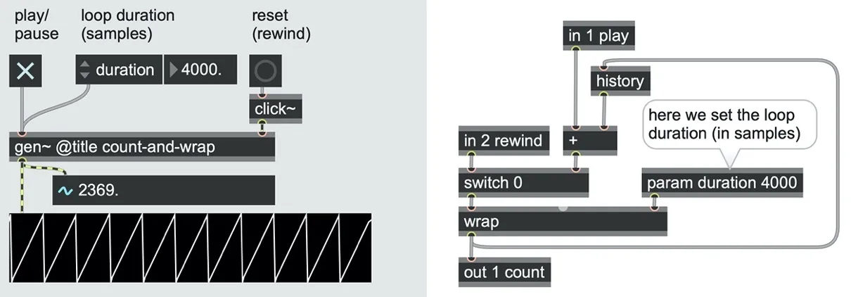
counter_and_wrap.maxpat

In this patch, we started with our initial accumulator-based patch. We inserted a wrap operator inside of the feedback loop, using a param duration 4000 operator to specify the limit to which we wish to count. The lower limit inlet was left unconnected, so it will default to 0. Our accumulator works as we expect — it outputs number values between 0 and 3999, producing a nice ramp output, and restarts counting from zero every time we click on the button.

We can use this looping counter to loop the playback of a buffer wave file. All we need to know is how long the file is. Fortunately, the buffer operator in gen~ outputs the number of samples in any associated buffer~ object from its left outlet (and this will automatically update any time we change the buffer~ object’s content in the parent patch). So, all we need to do is to connect the buffer operator’s left outlet to the right-hand inlet of the wrap operator.

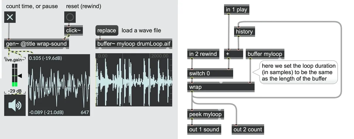
counter_and_wrap_buffer.maxpat

Thinking in rates and changes of phase (phasor)

What if we want to play audio files at different speeds, not just 1:1, with their original sampled rate? Perhaps we want to play a sound file at different speeds to change its pitch, or maybe we want to synchronize several different sound files to all loop at the same tempo, regardless of how many samples they contain.

We can change the playback speed by changing how much we accumulate every sample frame of passing time. For example, if we added two on every sample, our playback would run twice as fast, and if we added 0.5 on every sample, our playback would run at half speed.

If we count by fractional numbers, our counter will output fractional sample counts. However, here we run into a problem. If, for example, our sample count is 1.5, then which sample slice should the peek operator fetch from the buffer? Since the peek operator can only read a whole number (integer) position from a sound file by default, the fractional information will be ignored.

For example, if we count by steps of 1.2 to play back at 1.2x speed, then every 5th sample point will be skipped (indicated by the grey boxes in the following table).

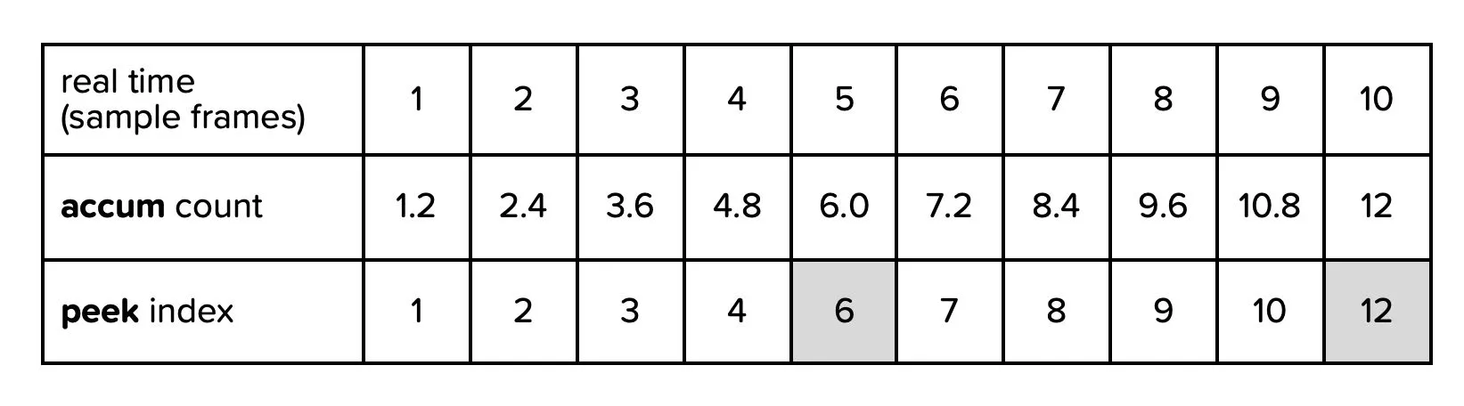
Unfortunately, this will cause an audible distortion (a kind of aliasing or nonlinear harmonic distortion). The usual solution to this problem is to apply some kind of interpolation when reading from the buffer. Interpolation just means estimating what the waveform’s position would be between sample frames.

The most convenient solution we can choose for now is to use a different buffer reading operator that automatically performs interpolation[19] when reading data: the sample operator. (We’ll be returning to problems related to aliasing distortion later in the book).

The sample operator also has another important difference. Rather than sending it a sample index to read from a buffer, we send it a phase. This simply means a floating-point number between zero and one that represents the relative position from the start to the end of the buffer. It doesn’t matter how many samples the buffer contains. It could be a hundred, or it could be a hundred thousand.

From the sample operator’s point of view, the phase is always just a normalized value between 0.0 and 1.0. Ensuring the 0.0 to 1.0 range is easy: we can modify our accumulator to use a wrap 0 1 operator.

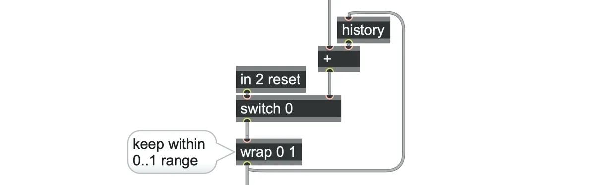
There is a very important implication for this change. It means that the duration of the loop is no longer determined by the amount of data in the buffer; it’s determined only by how we count. And that’s great because it means we can now set our looping to work with time scales we’re more comfortable with — say, in terms of seconds or milliseconds, or in terms of beats at a certain tempo, or as a frequency in Hz.

A phasor (using Hz)

If we’re no longer counting in samples, how do we know what to count by? Let’s look at an example working from a frequency in Hz. Remember that our accumulator is adding something to every passing sample frame of real-time. The number of sample frames of time in one second is simply the sample rate, which we can implement using either the samplerate operator or simply saying “samplerate” as an argument to another operator. If our sample rate is 48000 samples per second, and we want a loop that lasts exactly one second long; then, we want to add in steps that would reach 1.0 after 48000 sample frames. That means adding in steps of 1/48000. But if we wanted two loops per second (2Hz), we would need to count twice as fast, which means adding in steps of 2/48000.

So that’s our answer: for a given rate in Hertz, the amount our accumulator counts by (the change of phase per sample frame) is calculated as the ratio between our desired playback frequency and the system’s sampling rate: frequency / samplerate. This value is sometimes called the normalized frequency or the phase increment. In this book, we’ll often just call it the slope for short. We can now modify our patch to compute the slope from an input frequency by the sample rate using a / samplerate operator.

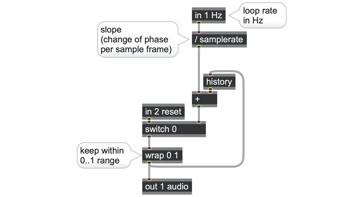
phasor_counter.maxpat—effectively the same as a phasor operator

The circuit we have just created is so useful that it also exists as a built-in operator: the phasor. The output looks like a sawtooth shape but is unipolar, rising from 0.0 to 1.0. In this book, we call these ramp signals or phasor signals.

Here is a ramp signal at 2Hz (two cycles per second).

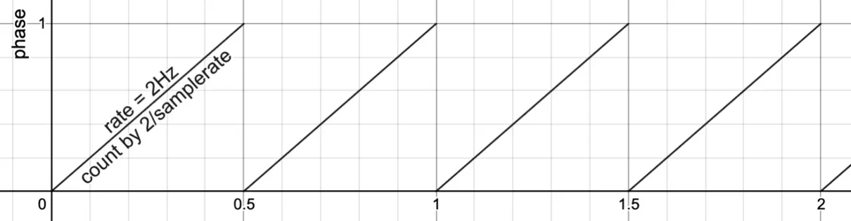
If we directly plug this patch (or an equivalent phasor operator) into a sample operator, we can get an oscillator whose waveform is defined by a buffer of data–sometimes called a wavetable oscillator.

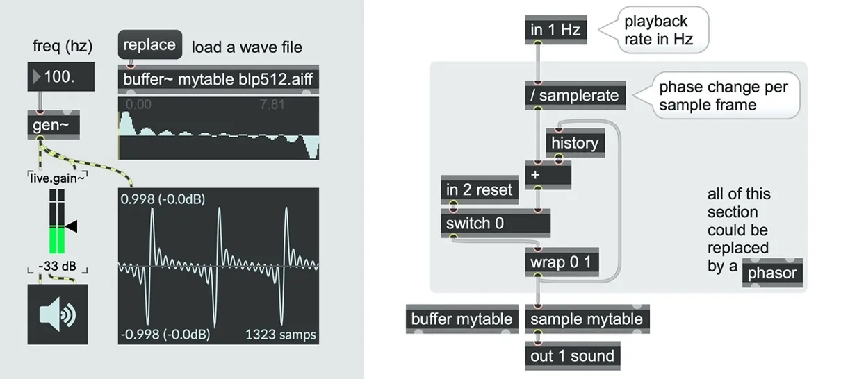
phasor_basic_table_oscillator.maxpat

It doesn’t matter how many samples are in the buffer~; the oscillator will always play at the frequency we set at our in 1. We can also dynamically replace the buffer~ contents, and this fundamental frequency will be maintained. Although this table-based oscillator is very simple, it is already very flexible. We’ll look at more powerful wavetable oscillators in Chapter 9.

A drum loop (using BPM)

The patch above uses a very short sound file, just a single cycle of a waveform. But we can replace the audio file with anything else that could loop, such as a breakbeat sample. Send a replace drumLoop.aif or replace jongly.aif message to the buffer~ mytable operator. You’ll probably notice that the playback will seem very rapid or sound quite complex and noisy. The phasor patch is working perfectly fine, but the looping frequency is too high to hear the breakbeat. If we drop the playback frequency down to around 0.2-0.5 Hz, we should start to hear a drum pattern looping nicely.

But it’s much more common to think of tempo in terms of BPM (beats per minute). If you want to specify a tempo in beats per minute, we need to convert a per-minute value (we’ll use a param bpm operator to set that value) into a per-second frequency for our ramp. Since there are 60 seconds in a minute, this just means dividing our BPM value by 60.

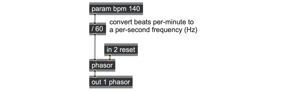
However, our drum loop or breakbeat might represent four, eight, sixteen, or some other number of beats. To get our desired looping rate, we also need to slow the phasor further by dividing the frequency by the number of beats per loop.

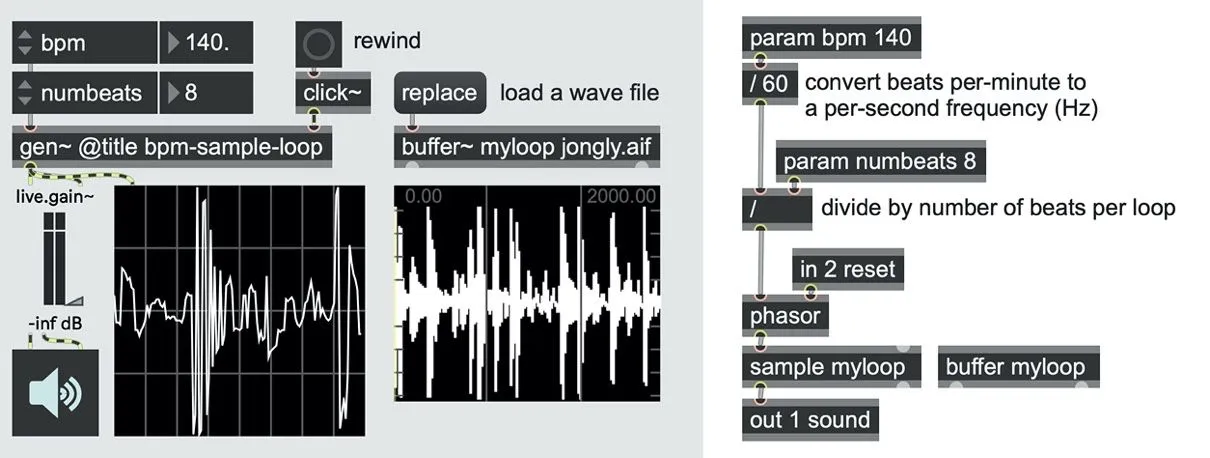
phasor_bpm.maxpat

Ramps as cyclical time

Let’s step back for a moment and consider how we represent rhythm as a signal.

Rhythms are often described as patterns of events. The events typically tell us when to hit a drum, start a new note, etc., relative to an underlying metric pulse, grid, or “beat” that is a regular and potentially endless sequence of evenly spaced instants, rather like the ticks of a clock. Here, for example, is the characteristic “Clave Son” pattern of five events over a grid of 16 pulses.

It’s easy to see why we might also gravitate toward thinking of musical pulse as a series of ticks or with empty space between them. This is how timing signals work in a variety of systems, from MIDI clocks, various forms of synchronization (DIN/SMPTE), as well as analog synthesis “clock triggers”. But is this really the best way to work with musical time?

Rhythm endures through time—not just when we hit things—just as time passes between the moments when the second hand ticks. In this book, we’re going to explore a different way of thinking about rhythmic pulse by expanding upon the phasor ramps we’ve already built in this chapter. We hope to show how phasor ramps can better capture the cyclic quality of rhythmic pulse as a signal.

To begin to explain why, let’s compare the two representations.

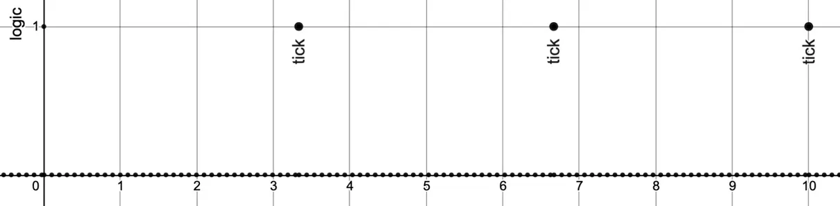Trigger-based clock: a periodic train of occasional single-sample impulse spikes (the “ticks”), with zero values filling all the durations between them.

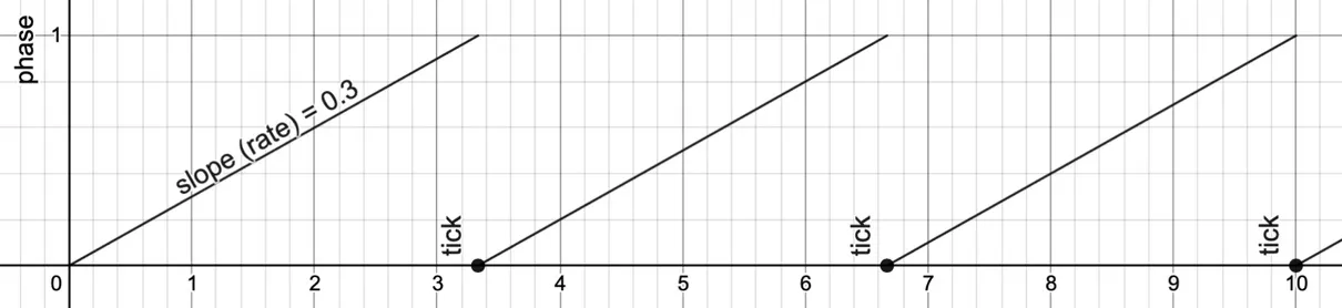Ramp-based clock: a continual signal at a given slope, in which the pulse is marked by when the ramp wraps around from 1.0 to 0.0.

Cycling ramp functions provide a precise, signal-based way of representing the continual passage of time. Unlike trains of ticks, a repeating ramp function conveys timing information at all moments between pulses, not just when the spike happens. This information includes

• The phase, which tells us exactly where we are between pulses,

• The rate or tempo (the slope of the ramp). This includes whether it is going in reverse (when the slope is negative) or is paused (a zero slope).

This information is also crucial when dealing with changing tempos. For example, in the following trigger-based graph, the tempo starts at about 20 triggers per second at the start and ends up at about 10 triggers per second at time = 1.0, but you don’t know how the tempo is changing until the next trigger comes in earlier or later than expected. Processes synced with this clock may also become sloppy.

In contrast, the ramp signal pictured in the following graph gives you an accurate representation of changing tempo all the time. The tempo is exactly proportional to the slope of the phasor. the steeper the slope, the faster the clock. And as you can see, this also includes representing clocks running backward (where the slope is negative, running downward instead of upward).

This is just one benefit. Knowing how time passes between beats was also essential for making our sample playing patch, and as we will see in this chapter, working with cycling ramps also allows a rich palette of signal-based transformations of rhythm that are far more difficult or impossible to achieve using triggers alone. (Later in the book, we will also see how cycling ramps can provide audio-rate timing accuracy that is better than sample-accurate–and why that is important.)

Exploration

To demonstrate, let’s start from the same breakbeat looping patch from a few pages ago (phasor_bpm.maxpat), which has a phasor clock that spans the entire loop (8 beats). We’re going to do some processing to the looping ramp at the heart of this patch before it reaches the sample operator for playback.

No matter what we do, the final ramp signal must still stay within the 0.0 to 1.0 range, so we’ll add a wrap 0 1 operator to ensure that.

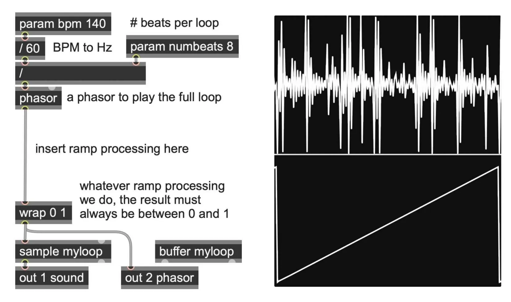
phasor_loop_processing.maxpat

Between the phasor and the wrap 0 1 operators, we can explore a wide range of different ramp clock manipulations. For example, we can try multiplications and additions.

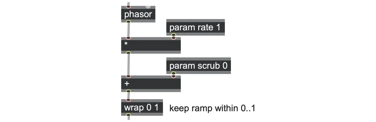
Adding (or subtracting) allows us to “scrub” the playback back and forth, but the playback tempo remains the same. Adding an offset to the phase like this is a really simple way to derive shifted rhythms like hocketing. Meanwhile, multiplying the clock signal lets us make things play faster or slower. Multiplying by two makes it loop twice as fast; multiplying by eight makes it loop eight times in the same period; multiplying by -1 makes it play in reverse. Multiplication is a really simple way to derive related pulses.

Example: beat slicing

Let’s plug these ideas together and build an algorithmic beat slicer. Imagine if the jongly.aif wave stored in the buffer is divided into 16 even slices:

We can define the number of slices using a param slices 16 operator (we can add an @min 1 to this operator since we can’t have less than one slice!)

These 16 slices span 8 beats of time over the whole loop. Now, every 16th of a loop (every half beat), we’d like to offset our sample playback to start at a different one of those slices. In order to fire events at every 16th of the loop time, we can run a second ramp 16x as fast as the loop phasor just by multiplying the loop phasor by the slices parameter and using a wrap 0 1 again to bring that back to the 0.0 to 1.0 range. This creates a ramp that loops 16 times as often, but since it also makes the slope 16x steeper, unfortunately, it also plays the sample 16 times faster too.

To get the original slope and sample playback speed back, we need to divide by the number of slices again.

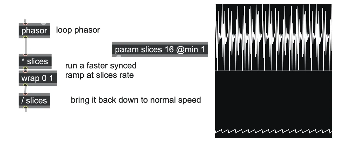
Now the ramp doesn’t go from 0 to 1. It goes only up to 1/16, and what you can hear is the first 16th slice of the waveform playing over and over. a 16th note repetition of the opening kick. Here we can bring the scrubbing idea back. If we add to our ramp before dividing by the “slices” parameter, we can select a different 1/16th slice of the waveform.

For example, picking an offset of 12 will jump 12/16ths into the waveform, repeating a high-hat sound.

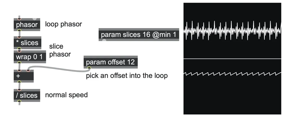
To get a precise slice, the offset should be a whole number (an integer). That’s easy to do by adding a floor or round operator after the param offset. You might notice that scrolling around the offset parameter can create a lot of clicks and noise as it continuously changes. To avoid this, we could use a latch operator to limit when parameter changes are passed through, and in this way, lock changes to the beat. The latch operator needs a trigger input to work but getting triggers from a ramp is simple: we are just looking for the moment when the ramp wraps around, which is the moment when the ramp’s change is very large.

The simplest way to find this moment is to check how much the signal has changed since the last sample frame, which we can get from the delta operator. During the ramp’s rise, this delta is a very small number, but at the moment it wraps, it is almost -1.0 (or almost +1.0 if the ramp was going backward). We don’t care if the ramp was forward or backward, so we feed the result through an abs operator to ignore the sign. Then we can use a > 0.5 comparator operator to detect when this delta is large and thus output a trigger signal with a value of 1.0 (true) when the ramp wraps and 0.0 (false) everywhere else; just what the latch operator needs.

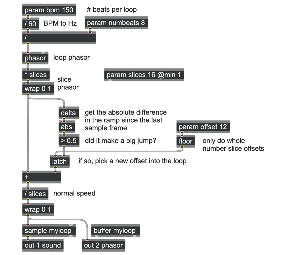
Now all we need for our algorithmic beat slicer is to replace the param offset with some process to generate the slice offset automatically. There are lots of different kinds of signals we could plug in here! For example, we could jump through the slices at different rates by further multiplying the phasor.

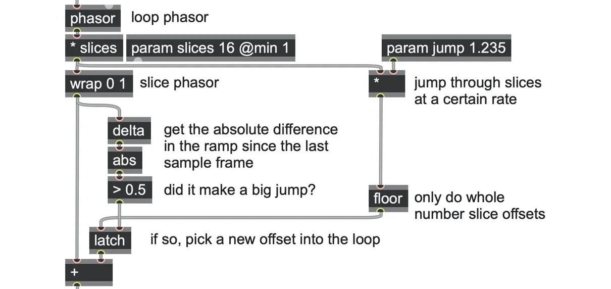
If the param jump is set to 0, we will be back to a single repeating slice. If the jump is set to 1, we’ll get a continuous playback of the whole loop. With param jump set to other values, we get different patterns of slices. Even fractional values do interesting things. We can add a little randomization to this, too–by mixing in a small amount of a noise operator to our jump signal. We’ll add the chance that we might pick the slice immediately before or after instead, adding some refreshing variation to the pattern to create our final patch.

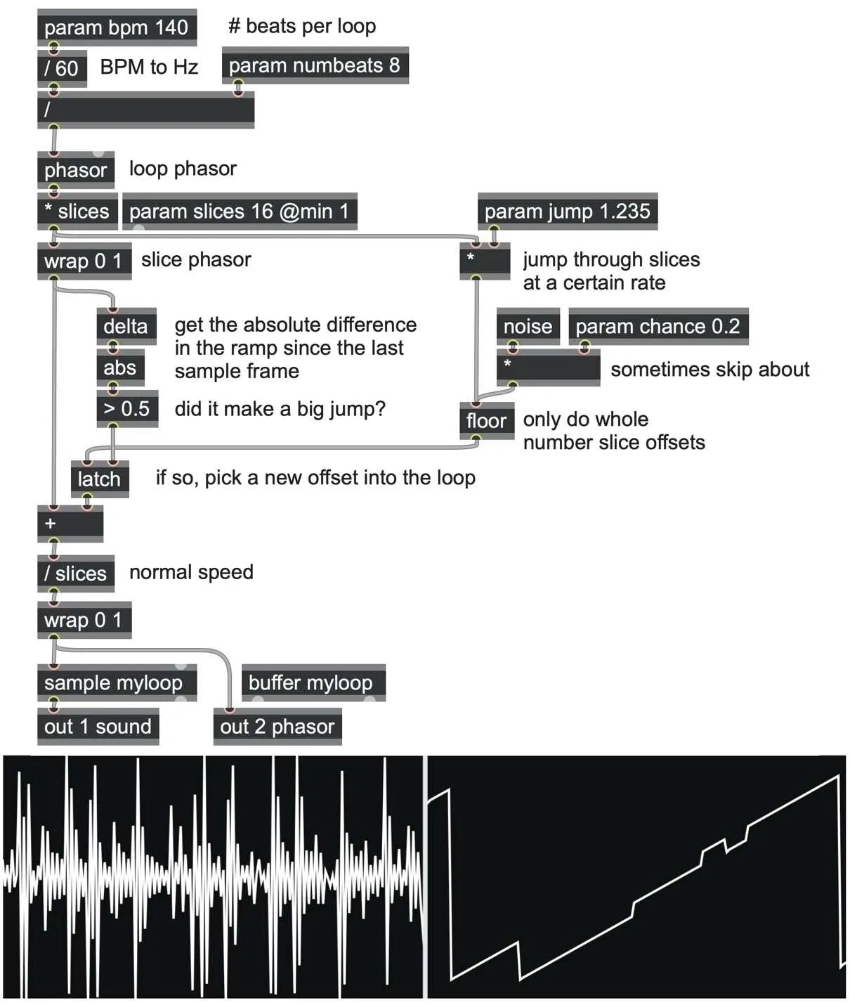
phasor_beat_slicer.maxpat

A collection of ramp processors

In the process of building the beat slicer, we encountered a few things that are worth looking into in more detail, which we’ll do over the next sections. Along the way, we’ll build up more abstractions that we will use throughout the book.

A phasor as a clock source

First, let’s build ourselves a primary clock generator. As we saw in the last section, we can use a phasor operator to generate a ramp at a certain BPM by dividing the BPM by 60 to get a frequency in Hertz.

When we built our counter-accumulator at the start of this chapter, we could pause its progress by setting its counter increment to zero. Pausing a phasor operator is just as simple: we can pause our clock by momentarily setting its frequency to zero (so that internally, it is counting by adding zeros). A simple way to do this is to multiply the frequency by a logic signal, which is either 1 to keep the original frequency or 0 to set the frequency to zero and pause the clock. We can turn any signal into a logic signal using a bool operator; if the input is 0, it outputs 0. If the input is any other value, it outputs 1. So, we added a param enable operator, converted it to logic using a bool operator, and multiplied this with the frequency to pause or continue the clock:

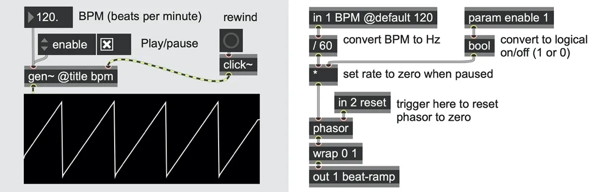
ramp_from_bpm.maxpat

Now that we have a basic clock source, let’s look at ways in which we can process the modular time of phasor-based clocks to do some more interesting things.

Ramp clock multiplication

Ramp multiplication is convenient when you want to derive multiple related clocks from a common source, such as measures and beats, polyrhythms, ratchets, and so on. Multiplying a ramp by any number greater than one will stretch it vertically: the period remains the same, but the amplitude, and the slope, are increased. For example, if you take a normalized phasor ramp, which runs from 0.0 to 1.0 (as with the dashed line below), and multiply the ramp by 4, the result is a ramp that runs from 0.0 to 4.0 and whose slope is also 4x steeper (as indicated by the solid line).

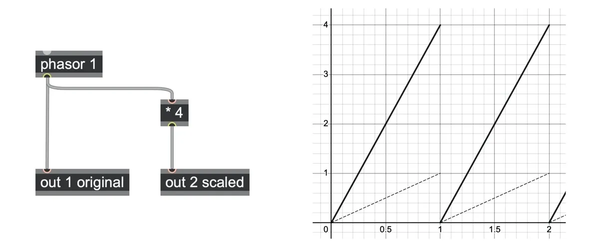
We can pass this scaled signal through a wrap 0 1 operator to recover a normalized phase range of 0.0 to 1.0.

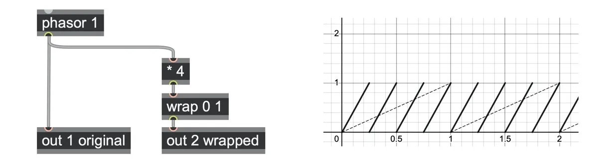
The slope is still 4x steeper, but now the period is 4x shorter. This makes sense: since the slope of a phasor is what gives its rate, increasing the slope means speeding it up, which means shortening the period.

In this way, ramps make it really simple to create precise substeps of any clock source, as opposed to a trigger-based clock world, in which clock multiplication requires quite complex and imprecise estimation.

We can use this to modify our ramp from the BPM patch to output both beats and measures. Let’s add a param beats operator to define how many beats there should be per measure (the upper number of the time signature in staff notation). Just as we did with the sample looper, we’ll divide our frequency by the number of beats to compute the phasor frequency per measure rather than per beat. Then, we can multiply the phasor output by the number of beats and feed that through a wrap 0 1 to get back our per-beat ramp.

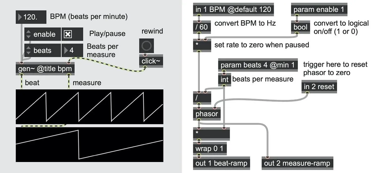
ramp_from_bpm.maxpat and go.ramp.frombpm.gendsp

If the input phasor is per beat or some other event level, then multiplication is an easy way to create ratchets. If the multiplier is a power of 2, you will get standard divisions (halves, quarters, eighths, etc.). If this is then scaled by 3/2, you will get triplet ratchets. Here is a variety of ratchet patterns produced by the ramp_ratchets.maxpat as an example:

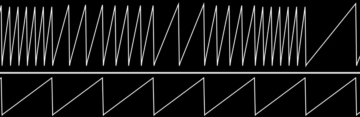
Using ramps as clocks also makes stranger fractional ratios of clock multiplications really simple. However, whatever fractional multiplier you use, it will be reset to the start when the input phasor wraps (whether this is the next measure, next beat, or otherwise). We will look at more free-running polymetric systems later in the chapter.

From ramps to steps

If we take a multiplied ramp through a floor operator, we will split it into a step function. For example, in the following graph, the ramp function (dashed line) is multiplied by 4, and then the floor taken to produce a step function of 0, 1, 2, 3, 0, 1, 2, 3 (indicated by the solid lines).

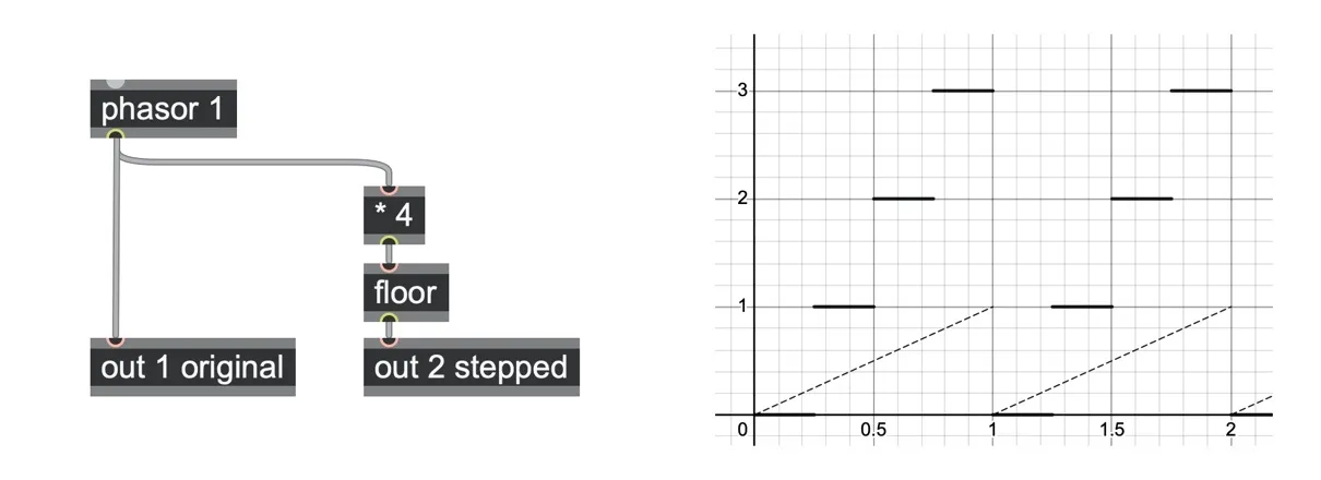
In this way, we can produce clock-synchronized step counts, which could be the basis for arpeggiation or other sequencing processes. For example, we used a variation of this in our beat slicing patch to compute the jump offset steps from a secondary ramp. If you want to normalize the steps to within a 0.0 to 1.0 range, just divide the step function by 4 again:

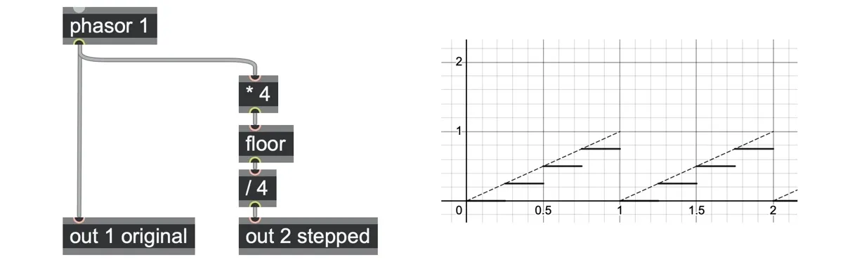
This sequence of multiply N, floor, and divide by N is at the heart of many quantization algorithms, and we’ll see it again in Chapter 5 among other places.

Putting all of these together, we have the very handy go.ramp2steps abstraction.

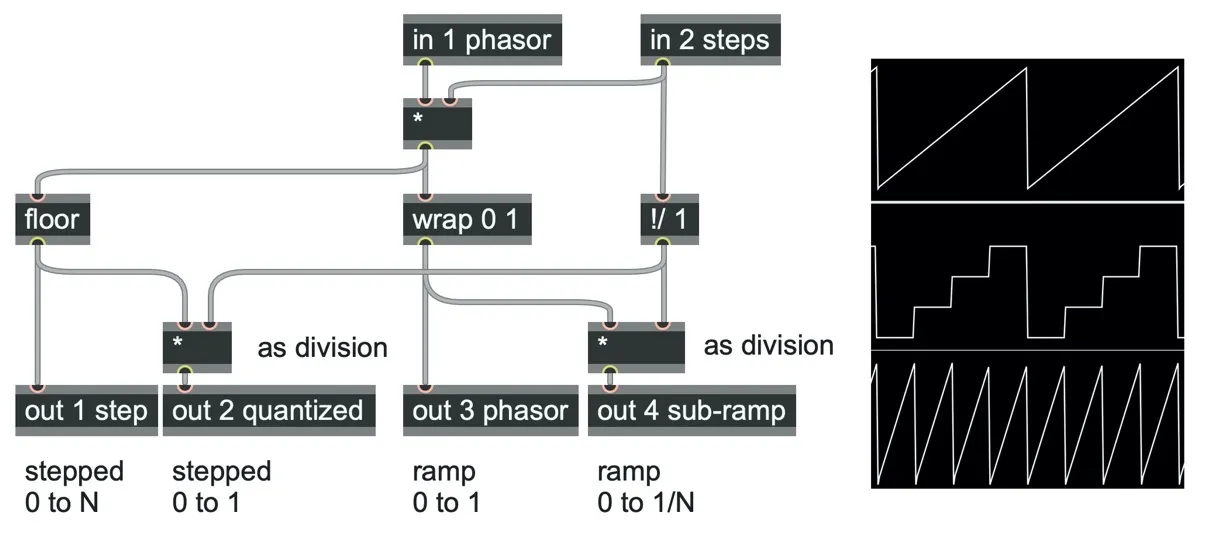
go.ramp2steps.gendsp

The ramp_steps.maxpat patch shows an example of adding two of these step functions together to generate an arpeggiated melody and multiplying percussion with steps to create accent rolls.

Shifting ramps (phase rotation)

One of the simplest manipulations we can make is to shift a ramp in time simply by adding or subtracting a phase delay (in 2 in the following patch) and then using another wrap 0 1 to bring it back into the 0.0 to 1.0 range. In the following image, the bold line is the original phasor, and the softer line is the same phasor delayed by 0.25 (25%) of a cycle:

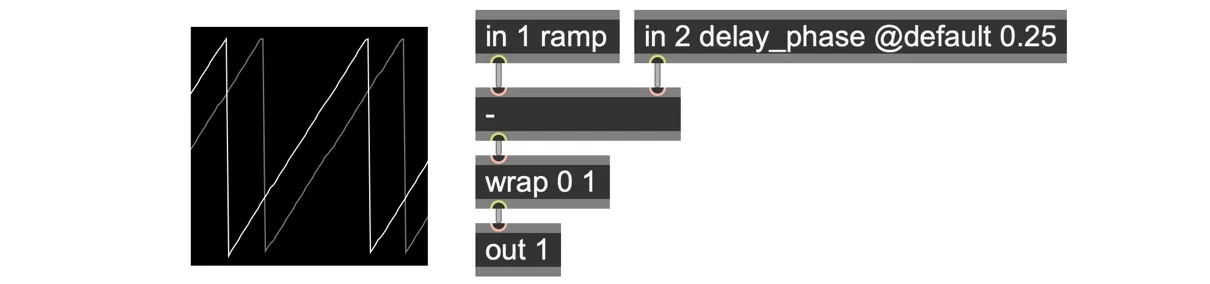
go.ramp.rotate

A phase offset by subtracting 0.25 will create a phasor that is 25% delayed. However, since phase is a circular concept, a phase offset of 0.25 can also be seen as 75% ahead (just as a 90-degree turn clockwise is the same as a 270-degree turn anticlockwise). Ramp shifting is, therefore, really phase rotation.[20]

The ramp_rotate.maxpat patch shows an example of driving two percussion patterns, one shifted relative to the other using a go.ramp.rotate abstraction. If the rotation amount is a very slow phasor, this can recreate the “phasing rhythms” characteristic of early Steve Reich compositions.

Getting the slope, frequency, period, and direction of a ramp

We can get the rate of change of a signal using the delta operator, which just subtracts the previous input from the new input (in mathematical terms, it is a discrete differentiator). If the input is a phasor or any normalized ramp signal, then this is almost all we need to get its normalized frequency (its “slope”).

There’s just one subtlety, which we can solve by applying a wrap -0.5 0.5 operator.

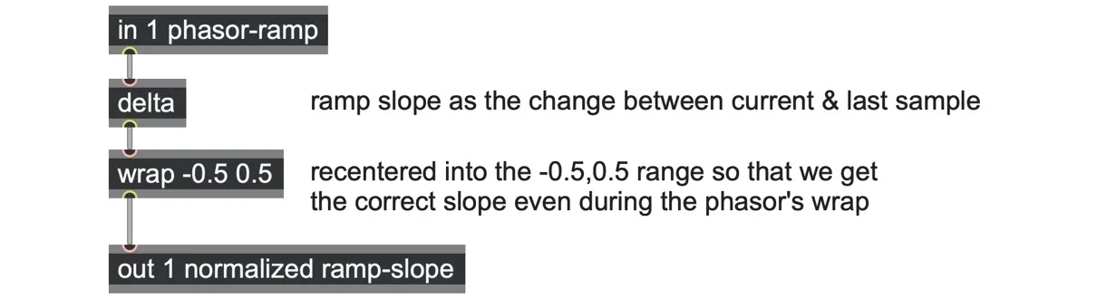
go.ramp2slope.gendsp

Why are we using the wrap operator here? Consider a looping phasor whose slope is +0.01 and whose bounds wrap at zero and one. When this phasor moves from 0.99 + 0.01 => 1.00, it will wrap back to 0.00, resulting in an apparent delta of -0.99. But wrapping that -.99 value between -0.5 and 0.5 will give us a value of 0.01, thus recovering our original correct slope. This also works for reversed ramps!

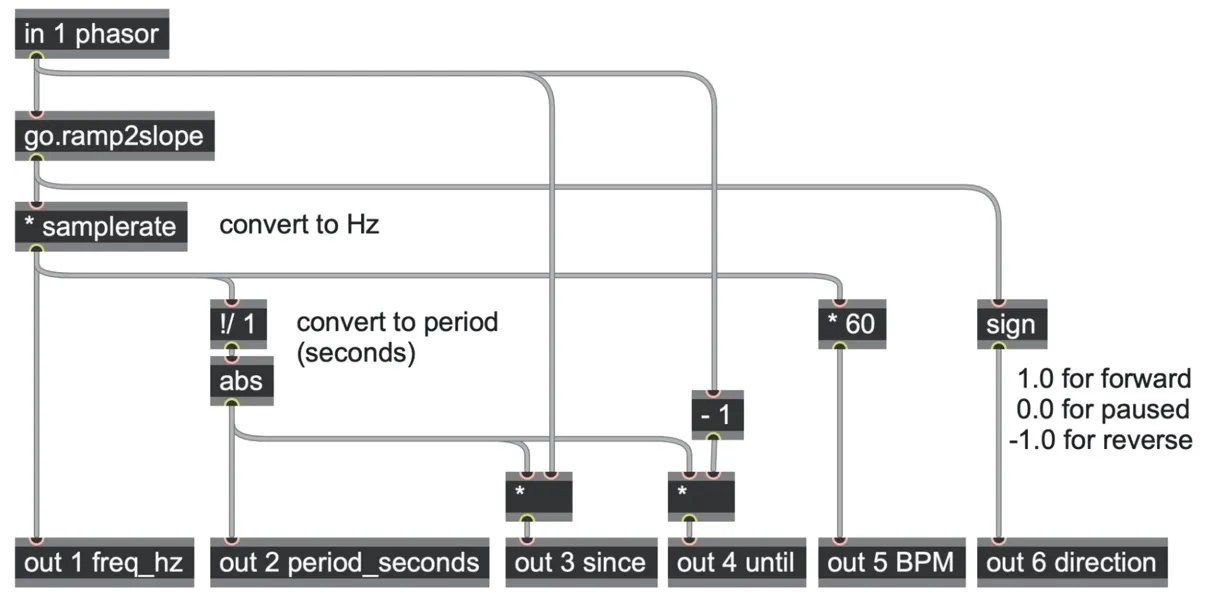
Now that we have the slope, we can derive all kinds of useful values from it—at any point in time!

• Would you like the rate in Hertz (cycles per second)? Just multiply the slope by the samplerate.

Do you want the rate as a BPM? Multiply the frequency in Hertz by 60.

• Do you want the period of the clock in samples? It is the reciprocal (one divided by, or !/ 1) of the slope.

If you want the period of the clock in seconds, it is one divided by the frequency (or feed the slope into a !/ samplerate operator).

• Multiply the period by the clock ramp, and it will tell you how much time has elapsed since the last wrap (assuming the rate is not changing). Multiply by clock - 1 to estimate how long until the next wrap.

• Do you want to know if the clock is running forward, backward, or paused? Look at the sign of the slope. It will be +1.0 for forward, -1.0 for backward, and zero when paused.

• Here are all of these things together in the go.ramp2freq.gendsp abstraction.

Getting triggers from a cyclic ramp

If you need triggers, perhaps to reset an accum operator for example, it is easy to get them from a ramp. It just means looking for the moment when the ramp wraps around. The simplest way to find this moment is to check how much the signal has changed since the last sample frame, which we can get from the delta operator. During the ramp’s rise, this delta is a very small number, but at the very moment it wraps, it is almost -1.0 (or almost +1.0 if the ramp was going backward). We don’t care if the ramp was forward or backward, so we feed the result through an abs operator to ignore the sign.

We can then use a > 0.5 comparator operator to detect when this delta is large and thus output a trigger signal with a value of 1.0 (true) when the ramp wraps and 0.0 (false) at all other times.

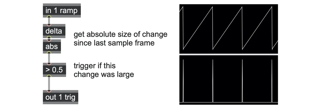
ramp_to_trig.maxpat

This concept is incredibly useful, and we use it throughout this book, so we created an abstraction for it called go.ramp2trig. But if you look inside go.ramp2trig, you’ll see the patch is more complex to handle a few subtleties. Let’s look at each one in turn.

The first subtlety is that resets to the input phasor do not always cause triggers. If the ramp happened to be reset during the first half of its duty cycle, the magnitude of change is not large enough to cause a trigger at that moment. We could perhaps reduce the threshold to something much smaller, such as 0.001 (which would detect resets so long as they are not in the first 1/1000th of the cycle), but then we run into the limitation that any ramp running faster than samplerate * 0.001 will start to generate spurious triggers. That might not be such a problem for tempo clocks, but it certainly can be for other processes!

Another challenge with this patch is that it will not give a trigger when a clock starts from the beginning. If you pause the clock, rewind it, then unpause, there should be a trigger at the moment of unpausing, but since at this moment the delta is very small, there will be no trigger.

We can address both problems by approaching wrap detection in a slightly different way. Rather than looking at the magnitude delta of the ramp signal, we can look at its proportional change. That means that instead of using the delta operator to get the difference between the current and previous sample frame’s magnitude, we get the proportional change by dividing their difference by their sum.

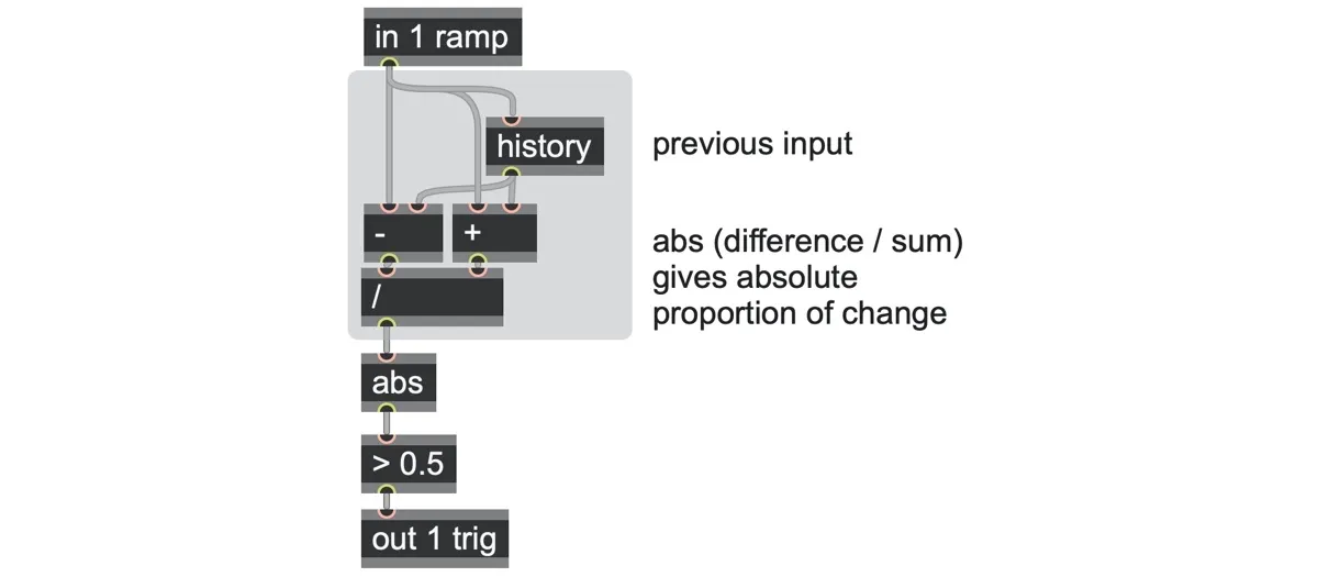
If the absolute proportional change is greater than the 0.5 threshold, we know that the input ramp is changing significantly, and so we send a trigger. In this way, any sudden kinks or significant changes in the slope of an input (such as happens when a phasor wraps) will output a trigger. In fact, a triangle wave will also cause a trigger. It also gives a trigger when the phasor begins from a rewound state.

The next subtlety is to prevent a trigger from being followed on the immediately next sample frame with another trigger. Here, we use a change operator into a > 0 operator to only output a trigger at the moment when the comparator switches to true.

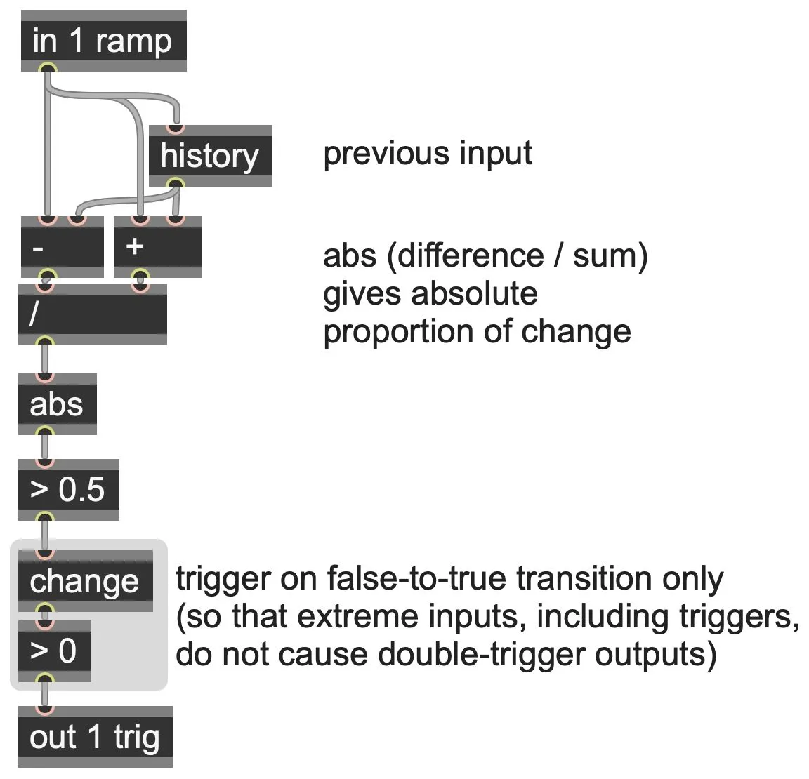
go.ramp2trig

This will prevent a sharp reset on the input from causing a double-trigger on the output, and also means the patch can process trigger-like inputs too!

Ramp/clock division

Earlier in this chapter, we saw how multiplication can create faster (shorter duration) ramps. In a similar way, division (or multiplication with a magnitude below 1.0) can be used to create slower (longer duration) ramps. However, we can’t simply scale the ramp itself, as it will never reach 1.0.

For example, if we scale a ramp by dividing by two, it will only run from 0.0 to 0.5. Instead, we have to create a second ramp accumulator and drive it with a divided slope.

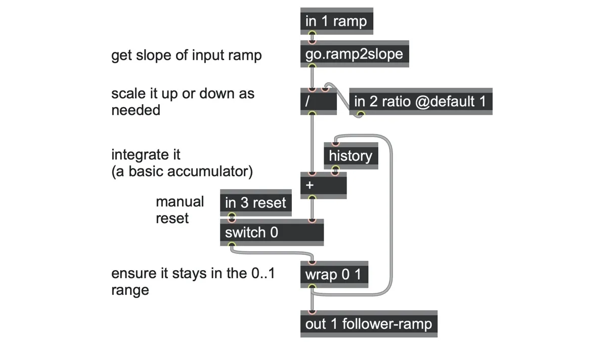
go.ramp.div.simple.gendsp

We take the rate of change of the incoming phasor, derived by using the go.ramp2slope abstraction, and integrate this slope via the same history, +, switch and wrap loop we saw earlier in this chapter. If the ratio is 2, then the output ramp will have twice the period (half the rate, which is to say, the clock divided by two) of the input ramp.

In fact, this patch serves a similar role as clock dividers in modular synthesizers, except that it works with ramps rather than pulses and thus can also clock divide at fractional rates with perfect precision.[21] Moreover, if the incoming ramp gradually changes slope, the derived slope immediately also changes accordingly; if the incoming phasor jumps, our derived slope will also jump by exactly the right amount.

Unlike the ramp multiplication we explored earlier in this chapter, we can work with divisions that are longer than the input ramp without being reset. However, even with simple divisions, with this patch, there’s no guarantee that the output ramp’s cycle will remain phase-synchronized with the input ramp. Even if they start synchronized, modulations to the ratio can cause them to drift. That might be desirable for some musical applications, but in the cases where it isn’t, the tricky part of clock division is how to sync the derived ramp: When should we perform the sync, and what do we sync to?

The go.ramp.div abstraction in the software included with this book tries to address this in a pragmatic way. This is a more complex algorithm than we’ve seen so far, but let’s go through how it works.

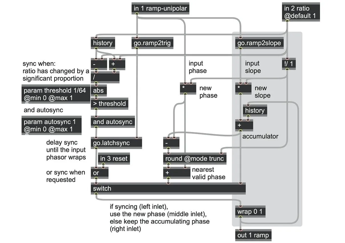
go.ramp.div.gendsp

The core circuit, shaded in grey, remains the same. We take the slope of the input ramp using go.ramp2slope, scale it by the divisor ratio to derive the new slope, and feed that into an accumulator built of history, +, switch, and wrap 0 1 operators. The main differences are the condition of when to sync and the determination of what to sync to.

When to sync: In addition to the manual reset input at in 3, this patch can also resync automatically if the in 2 ratio input changes by a significant amount. This is detected as a proportional change (in much the same way as we did for go.ramp2trig) by taking the absolute division of the difference and sum current and previous sample frame’s ratio values and comparing them to a threshold value (here via the > 1/64 operator). In this way, any gentle modulations of the ratio for tempo curves and so forth will not trigger a resync, but any sudden changes of ratio such as selection from a list will. (This can also be bypassed by setting the param autosync to 0 (off) via the and autosync operator.)

A request to resync here will not take place immediately, however. It is held inside the go.latch.sync abstraction until triggered by the go.ramp2trig abstraction when the ramp at in 1 cycles. This means that if you are working from a tempo clock input, the resync will happen at the start of the next beat or bar.

What to sync to: Rather than simply restarting the ramp at zero, we calculate what the real phase should be when the sync occurs by scaling the input ramp’s phase by the division ratio. That means we can even resync mid-cycle.

However, when dividing a ramp, there may be more than one viable place it could sync to. For example, a ramp divided by 4 has four possible beats it could align with. The go.ramp.div patch attempts to find the nearest viable alignment to minimize the change. In this patch, the trio of -, round, and + operators make it jump to whichever viable sync value is nearest.

Ramp multiplications and divisions with musical ratios

Musicians with training in Western systems may be in the habit of describing durations in terms of note values—as quarter notes, dotted eighth notes, triplets, and so on. This is easy using go.ramp.div.

Here are some examples of how to translate a ramp-per-beat (equivalent to 4n in Max time syntax) into different note durations.

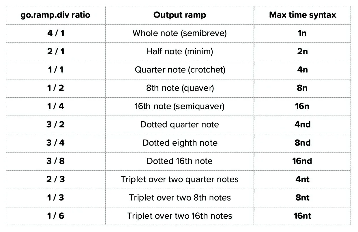
In the ramp_division.maxpat example we stored a list of common time divisions in the parent patch using a umenu object to select the desired division and a coll object to store the ratio parameters. This lets you choose common note values and shows you the numerator and denominator of the resulting ratios before feeding them to a go.ramp.div abstraction.

As an alternative, if you look at the first column of the table of ratios above, you can see it all comes down to simple integer ratios (simple whole number numerators and denominators). Moreover, there’s a simple pattern to them. Starting from a quarter note, we can multiply or divide by each power of 2 to get whole notes, half notes, eighth notes, sixteenth notes, etc. Then, to get a dotted note, scale by 3/2, or to get a triplet, scale by 2/3. For example, to get a dotted 16th note, we must scale by (1/4) * (3/2), which is 3/8.

If we could do these calculations within a gen~ patch it would allow you to make these selections algorithmically (and with sample accuracy). Here’s how these calculations might look:

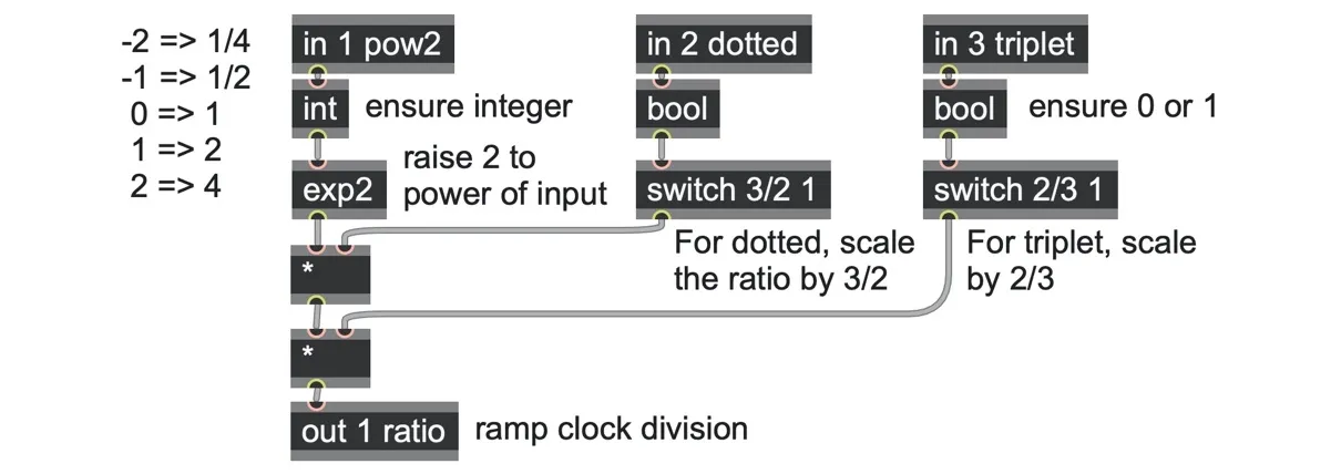
Once you understand the connection between note durations/tempo divisions and integer ratios, it’s easy to extend this idea to wider ranges of N-tuplets and other numeric patterns simply by choosing different numerators and denominators of a ratio directly. Working with simple integer ratios like this turns out to be very useful not only for calculating rhythms but also for other things like quantization, carrier & modulator frequencies for FM synthesis, and other processes we will see in later chapters.

Modular arithmetic with rhythms

We’ve now seen a couple of different ways that multiplying a ramp can produce related polymeters by subdividing a measure. But what if we want to break up a measure into sections of different durations?

For example, the 8-step pattern below, sometimes called the Tresillo rhythm, is one of the most widely observed rhythmic motifs spanning many cultures of music worldwide:

Amazingly, we can produce this easily with a bit of modular arithmetic. First, we multiply the measure’s ramp by 8 for the eight steps in the pattern and then use the wrap operator to get the remainder after division by three steps. That will produce ramps from 0.0 to 3.0, which we can normalize back to a 0.0 to 1.0 range by dividing by 3.

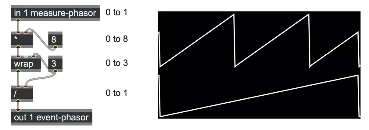
ramp.modulo.rhythm.maxpat [22]

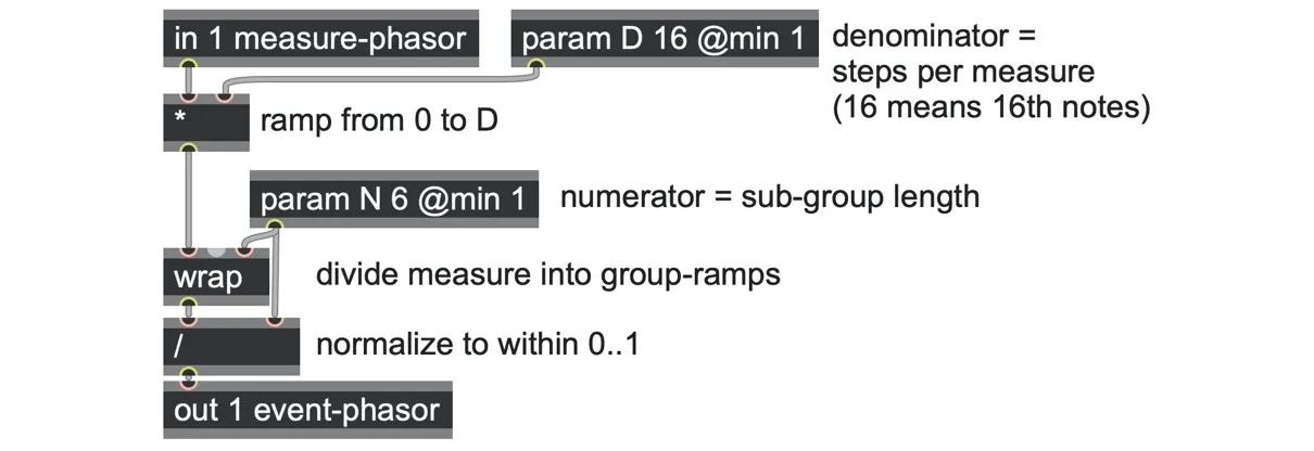
We can refine that patch beyond the 3:8 pattern to a more general N:D (numerator:denominator) pattern with param operators, as below. With this patch, you can explore a variety of different grouping patterns.

It gets even more interesting if you nest groups within groups: applying one modulo wrap operation for a first grouping level and then applying another, smaller modulo wrap operation for a sub-group level.

These parameters can be fun to modulate, so in the following patch, we also added latch operators to ensure that parameter changes are synced to the beat.

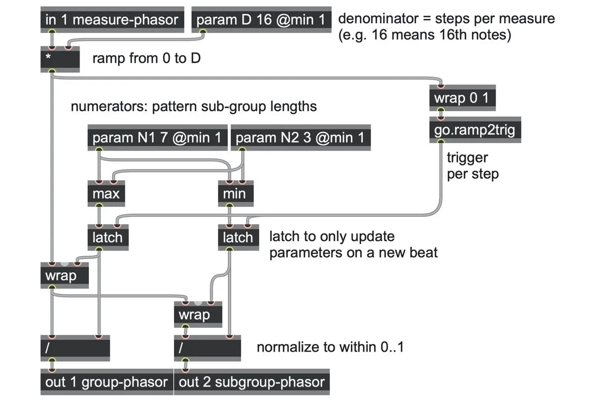
ramp_modulo_rhythm.maxpat

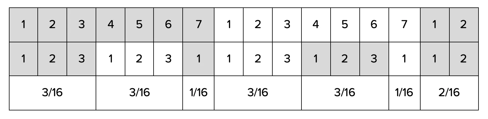
With the default parameters of 3:7:16, the resulting pattern looks like this:

Since these are all working with ramp signals, all the other things we can do with ramps work too. Here are the measure, group, and sub-group signals with a little swing added, using a shaping function we’ll introduce in the next chapter.

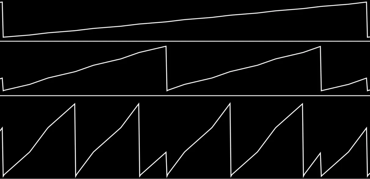
You can also feed this kind of ramp into the beat slicer to have more structured control! With a combination of the operations we’ve seen in this chapter and others we will meet in the following chapters, we can build up quite complex polyrhythms, and polymeters all derived from an underlying clock, and apply them to schedule all kinds of operations that work with triggers, step functions, or ramps, from triggering sound file playback, notes or other events, to driving LFO curves and sequencers, and so on. And everything is sample-accurate. Ramp signals really are one of the most versatile tools in your toolbox.

Modulating ramps with ramps

As a final example, let’s try something a bit more experimental. The go. ramp.div abstraction provides an easy way to stretch or compress the time of a phasor ramp. The ratio doesn’t have to be constant and can even be modulated continuously. What would happen if we modulated this ratio using another related phasor?[23] It may surprise you.

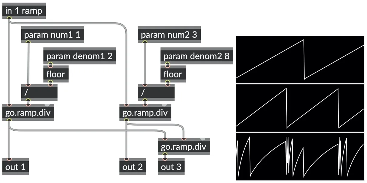
ramp_bursts.maxpat

The resulting waveform has become curved and tends to burst rapidly and then slow down, burst again, and so on.

If we wanted to get triggers from these bursty shapes, we could just route them through go.ramp2trig abstractions. To detect the kinks in the output (changes of slope), we could use a delta into a delta operator series, which gives us the equivalent of the acceleration of the waveform. This will provide us with spikes that are louder if the kink angles in the waveform are larger (and negative if the angular change goes down rather than up).

If we wanted to exclude the big phase wraps at the end of each ramp from this (since go.ramp2trig already finds those), we can use a go.ramp2slope into a delta operator.

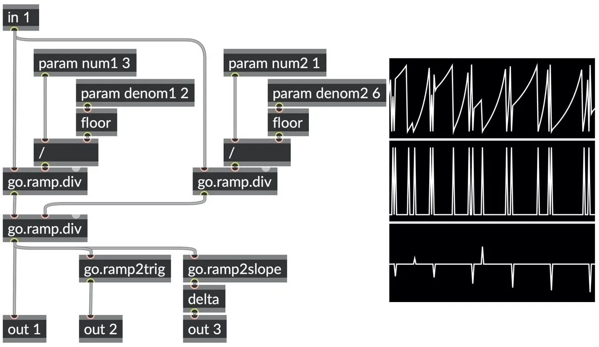
go.ramp_bursts2trigs.maxpat

To take the experiment to the next level, let’s insert a couple of LFO waveshaper operations just before our final go.ramp.div. We’ll add two pairs of unit shaper abstractions: a triangle operator with a skew param operator (to let us morph between positive ramps, negative ramps, and triangle waveforms) whose output is sent to a go.unit.lfo abstraction with a shape param operator (to let us morph between triangle, sine, and square wave outputs - we’ll build up this go.unit.lfo abstraction in the next chapter).

Here is a simple example of our now highly morphable waveform, and the very complex outputs it generates.

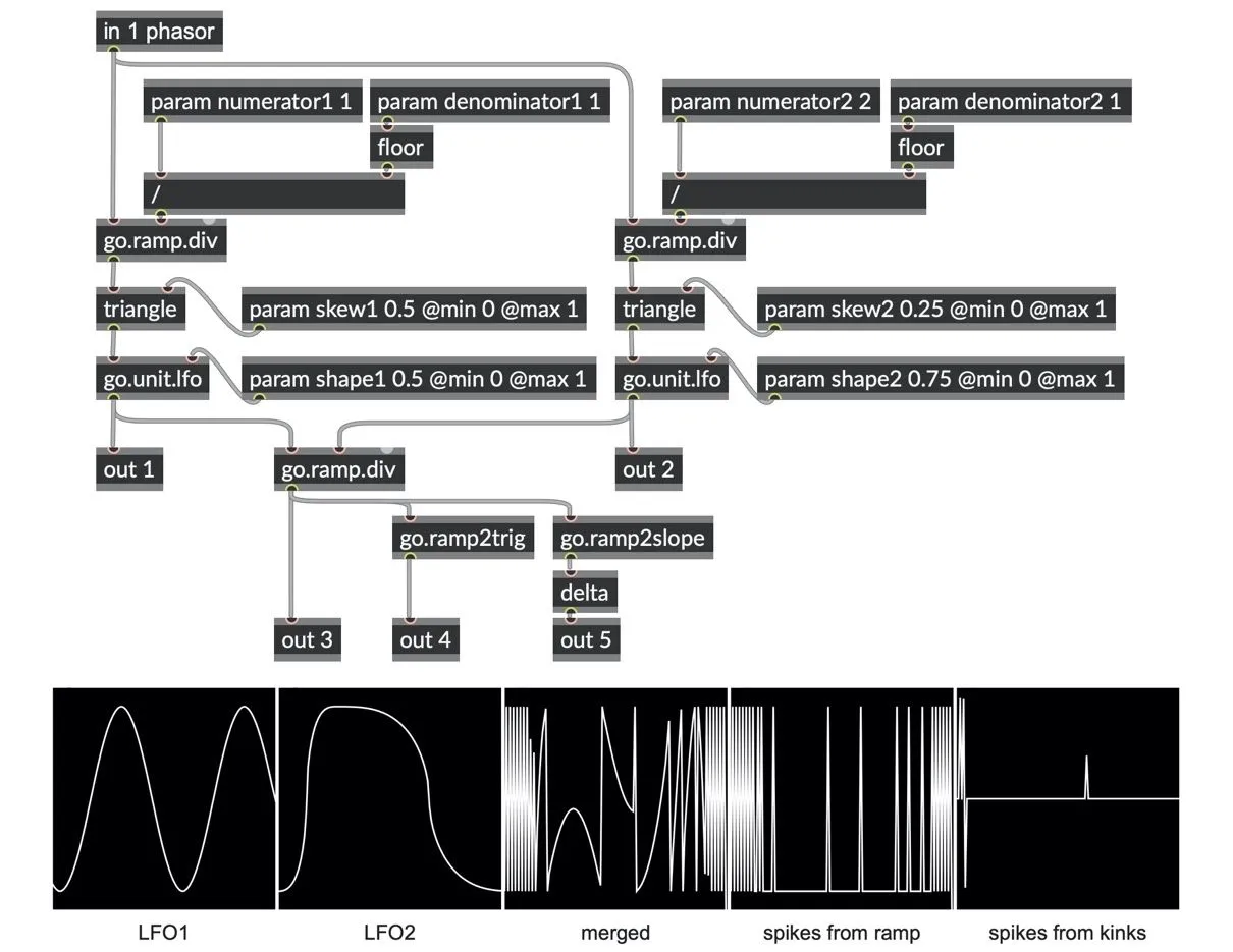
go.ramp_bursts_shaped.maxpat