Chapter 5:
Stepping in Time and Space

In this chapter, we will look at stepped signals and how they can be used for sequences of pitches and rhythms. This isn’t a chapter about how to play deliberately entered melodies, but rather an exploration of interesting methods to generate these kinds of patterns. Many well-loved sequencer circuits in the modular synthesis world can produce interesting rhythm and pitch sequences without ever having to enter a single note or step manually. Taking inspiration from these, we will look at ways to generate and transform interesting stepped patterns and how they can be used for pitches and other modulations of a sound.

Stepped pitches and logic gates

The way we think of sequencing is affected by our experience with music and the tools we use to make it. The realm of MIDI notes uses a paradigm inspired by pianos and Western music notation, in which variations of pitch and dynamics are synchronized together into a single message: much like a piano, a new pitch happens only when a new note begins. In the realm of modular synthesis, pitch and dynamics are typically represented as two independent signals, one for pitch and one for dynamics. Separating signals of pitch and dynamics allows their patterns to be defined independently, which, as we’ll see, opens up some interesting possibilities for generating musical complexity.

For example, if we were to graph the pitches of a monophonic melody we’re likely to get a stepped signal, where pitch values hold relatively steady for some duration and then jump to a new value for the next note, and so on (more or less).[41]

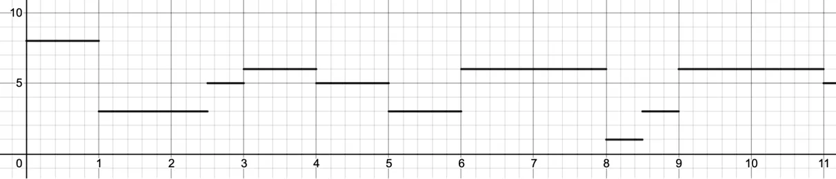
Most melodies don’t sound continuously; there can be rests or silences between notes. Graphing out whether a note is sounding or not also results in a “logic” or “gate” signal, where the value may indicate a note playing (being “on”) or a rest, where no note is playing (being “off”).

This kind of on/off logic signal is just about the simplest possible form of dynamics, but there’s still quite a lot we can do with it.

Creating step patterns by mixing logic signals

One of the simplest tricks to generate melodies in the modular synthesis world is to feed a few different logic signals into a mixer. That means, building a stepped sequence pattern by adding a series of related logic gate patterns at different levels. In a sense, it is a bit like melodic transposition—temporarily shifting a pitch from one basis to another—but in this case, we build the entire melody out of multiple overlapping transpositions at once.

This simple method can produce quite complex melodic patterns, particularly when the gate patterns loop with different durations (when they are polyrhythmic or polymetric). Here is an example of three gate patterns at different levels on the left and the combined complex pattern on the right:

We saw in Chapter 2 how we can build related rhythms from a single ramp source (such as a phasor operator) with the go.ramp.div abstraction.

The patch fragment above is an example driving 2nd, 3rd, and 5th divided ramps from a common phasor ramp clock. To turn these ramps into logic gate signals, we can use a comparator operator. For example, we can use a < (less than) operator to send a gate high for the first portion of a ramp:

Each of the gate signals should then be multiplied (attenuated or amplified) by a specific parameter level, and the sequencer outputs the total sum of these scaled gate patterns as an evolving “melody”. Here is all that put together:

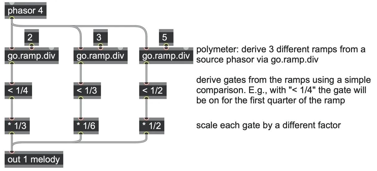
mixer-sequencer.maxpat

In the mixer-sequencer.maxpat patch, we map the output as a pitch value to set the frequency of a sine oscillator, but—of course—it could be mapped to pretty much anything you like.

Sample and hold patterns

Another common technique for generating a stepped signal sequence is to route the output of an LFO, envelope generator, or noise source (or any other signal) through a sample and hold module clocked by some rhythm or meter. Despite the simplicity of this technique, the results are a great starting point for modulation and experimentation.

We can use the latch operator to sample and hold any signal value. The latch operator’s left input is the signal to sample. The right input is a logic switch control which either allows the left input through to the output or holds the previous output constant. Any nonzero (true) value here will let the input signal through, while a zero (false) input value makes the latch continue to output the same value as it did on the previous sample frame. If the right control input is a trigger signal (i.e., mostly zero values with sparse single-sample spikes), then the latch operator acts just like a classic sample and hold module.

So, all we need to start constructing all kinds of interesting step sequencers is:

• A source to sample: some arbitrary curve, such as an LFO we created in Chapter 2.

• A rhythmic trigger sequence, such as we generated from ramps using go.ramp2trig in Chapter 2.

• A latch operator.

The latched-sequencer.maxpat patch shows a simple example: A phasor-driven LFO on the left producing a sine wave is latched by a different phasor-driven clock on the right.

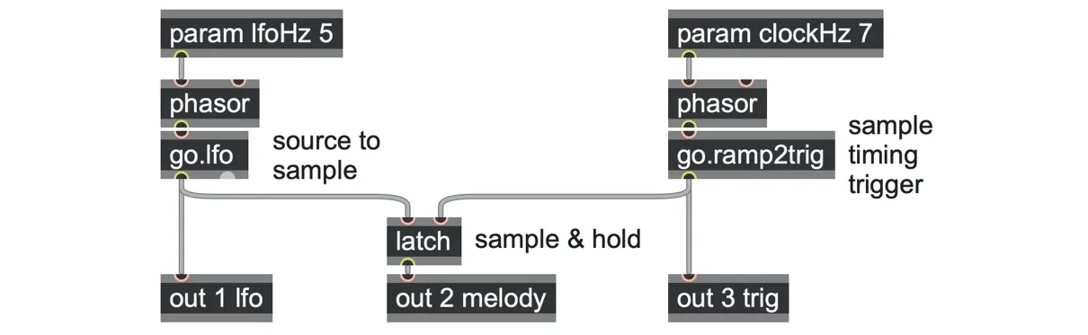
The output is shown in the following graph. The dashed line is the source (the go.lfo sine wave), the dotted line is the rhythmic trigger (the go.ramp2trig output), and the solid lines are the output values of the sample & hold latch operator.

Try setting the LFO rate to some multiple of the clock rate. If the LFO rate divided by the clock rate is a simple ratio, it will produce a static repeating sequence.

In fact, the length of the resulting sequence will be equal to the denominator of the smallest whole number equivalent to the original ratio. For example: If the LFO rate is 42 Hz and the clock rate is 4 Hz, then the ratio is 42:4, which can be reduced to the ratio of 21:2. The denominator of this ratio is 2, and—as expected—the sequence repeats every two ticks of the clock. If you change the LFO rate to 43 Hz, the resulting ratio of 43:4 can’t be reduced any further, so the sequence loop length is four steps.[42]

However, if the two rates do not easily reduce to a simple integer ratio, then their proportions are inharmonic, and the sequence will evolve over a very long time. It might have short repetitive fragments, but these fragments will seem to shift gradually in a way somewhat analogous to beat frequencies and musical phasing. These results can provide a rather interesting source of variety.

Note that the output of this sequencer can be any numeric value that the LFO (or another source) produces; you might want to quantize this into a set of specific pitches. We’ll come back to pitch quantization toward the end of this chapter.

A shift register canon

We can expand this patch to create the signal equivalent of a musical round, or canon, by chaining two or more latch operators in series using history operators.

go.shiftregister2.gendsp

We saw some patching like this in Chapter 4, where we used a latch/history series to generate random signals that smoothly interpolate from older to newer values, and we called it a “shift register.” That’s just a technical name for a kind of sequence of stages, each of which stores a value passed down from the previous stage. Here is an 8-stage shift register:

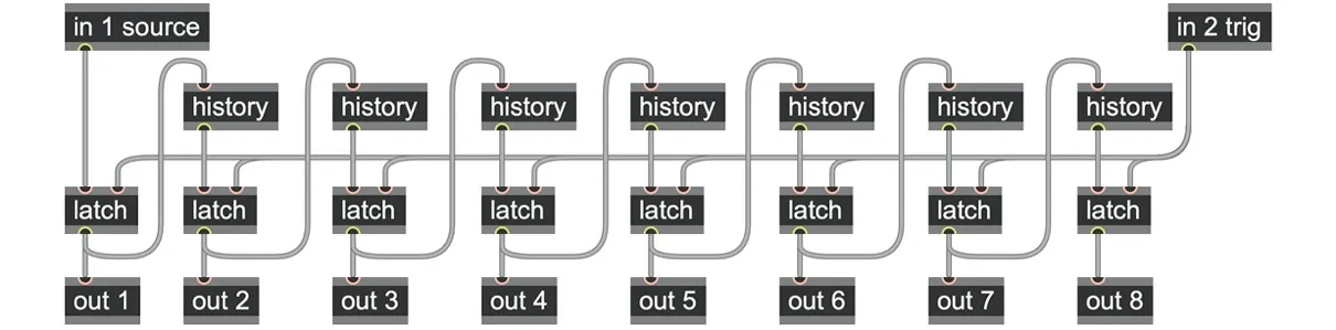
go.shiftregister8.gendsp

The layout of these stages resembles a “bucket brigade”: at each step of a clock, the values are shuffled down one stage in the brigade, and a new value is inserted at the front. That is, on every trigger (nonzero value) received at in 1, the left-most latch (the one above out 1) will sample a new value from the input source at in 2. However, its previous value, which was cached by the next history operator, will be passed along to the second latch (the one above out 2). Similarly, the previous contents of that latch operator will be passed along to the latch above out 3, and so on, cascading down to the rightmost latch. As a result, an input trigger causes the values of all the latches to shuffle one step to the right.

This is a general form of a shift register is also known as a FIFO—First In, First Out sequence—and thus is also a very simple kind of delay. The value sent from out 8 will be the same as the value sent from out 1, but delayed by the amount of time it took for seven more triggers to be received at in 1.

That delay also makes this bit of patching a generally useful tool for any situation where we want to work with any prior values at a given clock rate. We can also use this algorithm as a general kind of stepped delay in situations where we want to duplicate delayed copies of a stepped sequence that we can route to different purposes. For example, we might route delayed pitch sequences to different oscillators to create musical canons or route modulation sequences to different filter cutoffs, amplitudes, and so on.

For the following patch, we feed a go.shiftregister8 abstraction with a simple triangle wave LFO. The first stage of the shift register creates a pitch sequence by sampling and holding that input whenever the go.ramp2trig trigger fires. Each subsequent stage of the shift register creates a delayed copy of this pitch sequence.

To demonstrate the effect, the first and last stages are fed to oscillators (sounding like a canon or pseudo-delay effect) and visualized in scopes.

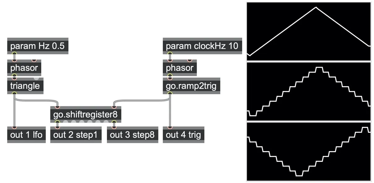
shift-register.maxpat

In the image above, the top scope shows the LFO waveform (the triangle wave at 0.5Hz) that is being fed into the go.shiftregister8 abstraction. The middle scope shows the first stage of the shift register (the first latch operator), as it is clocked at a rate of 20Hz. (So far, this is much the same as we did for the sample and hold sequencer at the start of this chapter.) The bottom scope shows the output of the final stage of the shift register (the eighth latch operator), which is a copy of the first stage delayed by seven clock triggers.

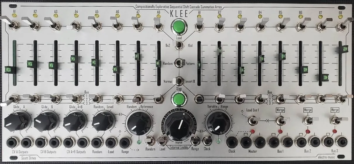
The Klee Sequencer; photo courtesy of Wiley Abt

Sequencing algorithms with binary shift registers

Shift registers also turn out to be at the heart of a number of popular and revered sequencing modules in the modular synthesis world — Scott Stite’s Klee sequencer (pictured above), Ken Stone’s Gated Comparator and Infinite Melody, Rob Hordijk’s Rungler & Benjolin, Tom Whitwell’s Turing Machine, and Mutable Instruments’ Marbles, to name a few.[43] All these modules build their complexity out of shift registers.

In hardware, the equivalent of a latch/history operator chain circuit is sometimes called an analog shift register, since it can store and pass down any voltage value. A digital (or binary) shift register is even simpler since the values stored in each stage are only a single binary bit: either zero (false) or 1 (true). Most of the hardware shift-register sequencers we mentioned above are in fact digital shift registers.

All this means for our purposes here is that the input signal on the left should be a logic gate signal of either 0 or 1, such as is produced by any comparator operator. We could, for example, compare a phasor ramp against a threshold of 0.5 using a < 0.5 operator for an alternating 0, 1, 0, etc. series.

That also means that the output of the latch stages are logical signals, either zero or one, which we can combine to produce interesting stepped signals. Just like the mixer-sequencer patch we saw in the first section of this chapter, we can multiply each of these logical signals by an arbitrary “weight” or voltage that is assigned to it, and the final output is produced by summing all of the weighted logic patterns together. In the shift-register-weighted.maxpat patch, we used an 8-channel buffer operator’s channels to retrieve a unique weight for each stage:

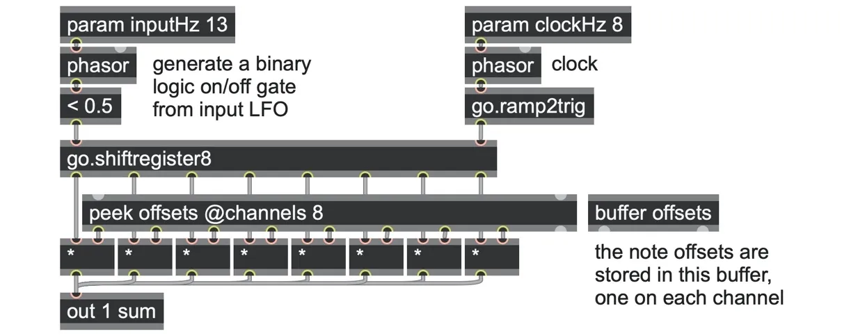
shift-register-weighted.maxpat

This technique can produce really complex sequences even if only a few steps have nonzero weights. Assigning negative weight values can make it even more interesting. As with the sample & hold sequencer, choosing a phasor frequency that is a simple multiple of the clock frequency will produce repeating cycles, but choosing a phasor frequency that is inharmonic to the clock rate will produce an evolving melody built out of common pitch offset fragments and motifs.[44] sAs an alternative, we could drive the shift register with a probabilistic gate input. For example, we could compare a noise source against a threshold parameter, just as we did with the go.chance abstraction in Chapter 4:

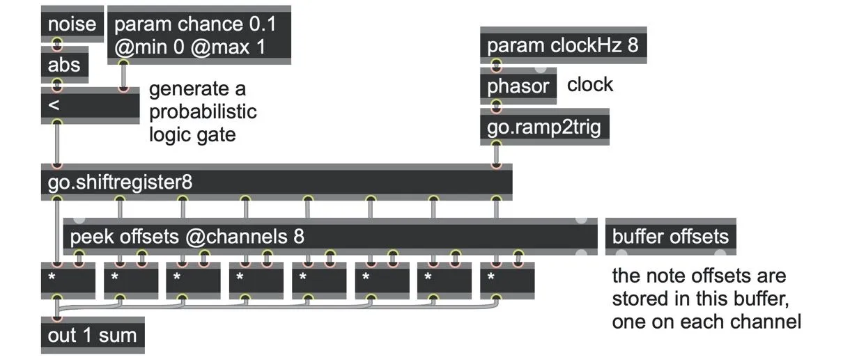
shift-register-weighted-random.maxpat

With a param chance probability of 0.0, you will hear a steady output at zero, as no data is flowing into the shift register. Raising param chance to 0.1, you will begin to hear a copy of the motif pattern stored in the buffer play through from time to time, and sometimes you will hear several of those motifs overlapping each other as a more complex phrase. Turning param chance up to 1.0 also produces a stable state, but this is because every single step is now overlaying the full motif. The most unpredictable patterns occur when param chance is at 0.5, with many random overlaps.

Looping

What if we heard a fragment of this random sequence that we like–can we modify the patch to keep a pattern looping, rather like we did for the Urn patch in the previous chapter? To keep any shift register looping forever, all we’d need to do is take the output of the final stage and feed it back to the input of the first stage. But then we’d lose the use of the original input, which we needed to get a pattern going in the first place!

One way we could solve this is to add some kind of switch to determine whether the shift register should use the live input or the looping feedback. We could even use a param chance operator and a random choice whether to loop or feed back.

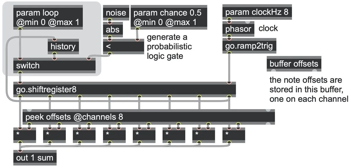
shift-register-weighted-random.maxpat

Evolving loops

If we did feed the last stage back, rather than just looping directly, we could feed it through some other logic operation to make the loop more complex. For example, if we use a not operator, the binary pattern will be inverted each time it passes through the loop, so we’ll alternately play the pattern and then play back its logical inverse (effectively doubling the loop length).

Tom Whitwell's Turing Machine and Mutable Instruments’ Marbles modules have a single parameter (called “déjà vu” on Marbles) that cleverly combines control over looping, inverting, and probabilistic choice. There’s a quite neat trick we can do to our patch to achieve the same thing—and all it takes is adding an xor (exclusive or) operator!

What is an exclusive or? It is one of the most fundamental logic relations, along with and and or:

• The and operator returns true (1.0) only if both of its inputs are true (nonzero).

• The or operator returns true (1.0) if either of its inputs is true (nonzero).

• The xor operator returns true (1.0) if only one of its inputs is true (nonzero) and the other is false (zero).

Let’s think about what happens if we feed our pattern back through the xor operator under different inputs, like this:

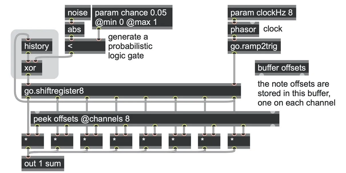
shift-register-weighted-xor.maxpat

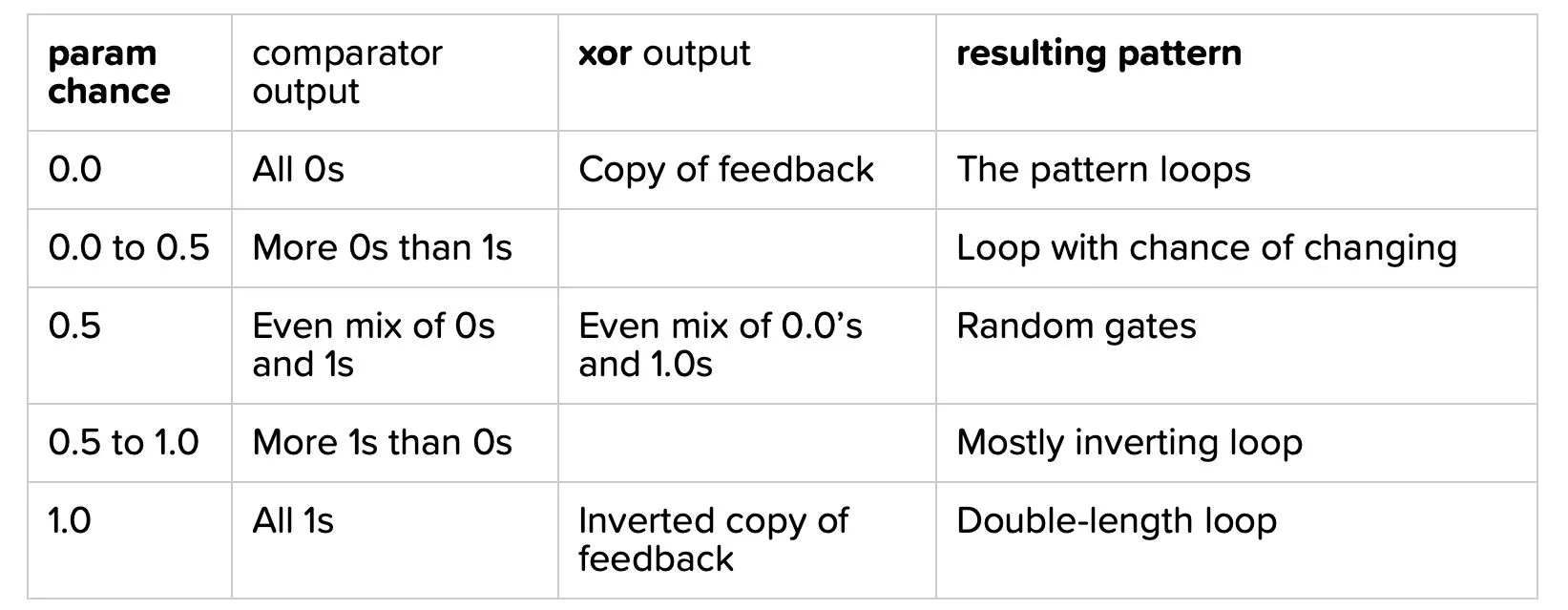
Imagine we already have a pattern going, and we set our param chance to zero, meaning the input signal is also always zero (false). Wherever there is a 1.0 in the feedback signal, the xor will output 1.0; wherever there is a zero in the feedback signal, the xor will output 0.0. That is, with param chance set to zero, the xor output copies the feedback signal, and our pattern will repeat in a loop.

If we set our param chance to 1.0, then the input signal will always be 1.0 (true). Now, wherever there is a 1.0 in the feedback signal, the xor will output 0.0, and vice versa: the xor operator inverts the feedback signal! In this case the pattern plays a normal copy and then an inverted copy, for a total loop twice as long.

For any value of param chance between, we will have some probabilistic chance of either copying or inverting the pattern. Essentially, the param chance sets the probability of the next step inverting. If the param chance is exactly 0.5, where any step is equally likely to copy or invert, we will get an entirely random sequence.

So, with just one xor operator and a probability input, we’ve replicated the full set of random pattern looping capabilities.

Using xor for pseudo-random sequences

Some interesting longer loops can also happen if we replace the probabilistic gate by feeding back another stage of the shift register to the xor operator instead. These kinds of circuits are called "linear feedback shift registers" (LFSRs).

For example, here’s an example takomg the xor of the 3rd and 8th stages of our go.shiftregister8, which ends up creating a sequence that repeats every 217 steps! All it needs is one bit pushed in at the start to get it going, which we do in this patch using an elapsed and == 0 pair of operators:

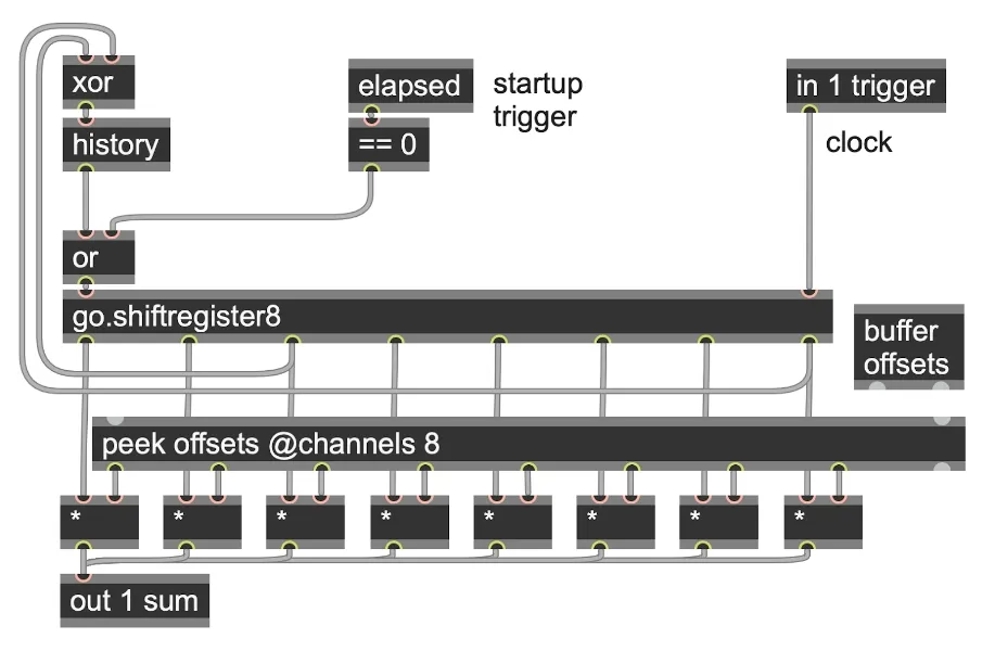
shift-register-weighted-xor.maxpat

Not every pair of outputs will give the same sequence length. For example, the xor of the 4th and 8th outputs has a sequence length of only 12 steps. Some combinations can give even longer outputs; for example, combining the 3rd, 5th, 6th and 8th outputs through xor operators (in any order) will give a sequence length of 255 steps; the longest possible sequence an 8-bit shift register can produce. Such "maximal length" sequences have a very even statistical distribution, and this makes them attractive as pseudo-random number generators. (In fact, the noise operator is based on a far more complex example of the same basic principle.[45])

The Buchla 266 Source of Uncertainty synthesizer module from the mid 1970's used a 6-stage digital shift register to produce pseudo-random signal sequences, including both a gaussian distribution by summing all the stages, as well as an even distribution through binary decoding, as described in the next section.

Binary decoding

Many of the hardware shift-register sequencers mentioned earlier don’t even have control knobs for the mixer weights: instead, the weights of each stage are fed into a “digital-to-analog converter,” or DAC, which produces a binary-encoded integer at the output. All this means is that we take each individual stage’s value—which is either “on” (1) or “off” (0)—and multiply it by a corresponding power of 2 (20, 21, 22, 23, 24, etc.). So the weights start at 1 for the first stage, then 2 for the second stage, 4 for the third stage, then 8, 16, etc., and all of these results are added up for the output value. That is, a DAC is really nothing more than a special case of a mixer in which the mixer levels are a series of powers of two, and the mixer inputs are binary gates. Another name for that is a binary decoder.

Here is what our random looping shift register from the last section looks if we convert it to feed an 8-stage (or 8-bit) binary decoder:

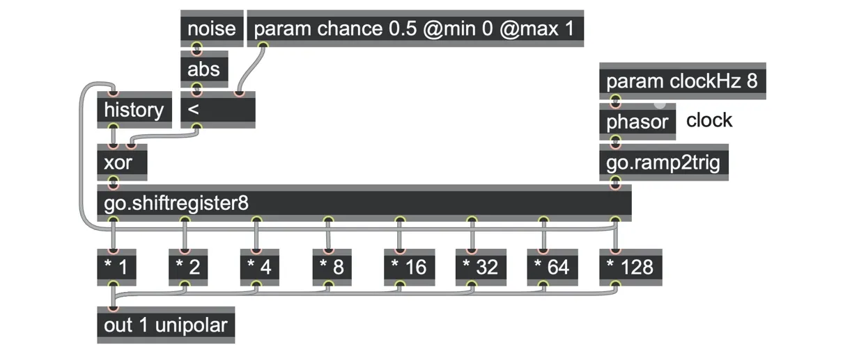
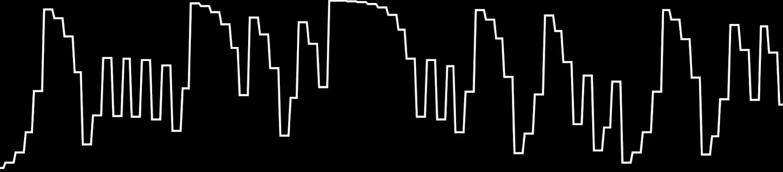
Since the shift register is being fed by a completely random input, you might expect that the output patterns are completely random too, but that’s not quite the case. Interestingly, the nature of shifting the bits tends to produce a lot of ascending or descending series, as well as other recognizable motifs:

An 8-bit decoder can produce an integer output from 0 when all gates are zero, to 255, when all gates are 1. (That limit of 255 is in math terms, 28-1, or in code terms, exp2(8)-1.)

What can we do with this integer value? We could scale it down to a useful range by dividing the result by 255, which would give us a unipolar normalized signal in the range of 0.0 to 1.0. Or we could scale it to some other useful range using a scale operator, and quantize that to select from a set of pitches, for example.

Integers as patterns

This brings us to an important feature of binary encoding: every different possible sequence of bits (the pattern of gates) encodes a unique integer, and vice versa: every integer encodes a unique gate pattern. Put another way; both the binary gate pattern and integers are two representations of the same thing. That means that the entire pattern can be represented as a single integer at any time.

This suggests the idea that the same results could be produced just by a few operations on integer signals rather than shuffling gates through a series of shift registers. Rather than using a chain of latch and history operators, we could simply apply numeric operations on a single integer at each clock trigger. But which numeric operations?

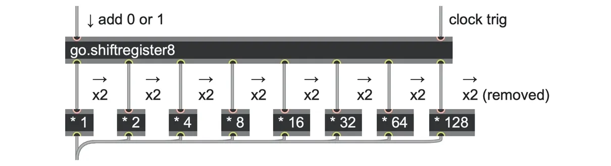
If you look at the 8-bit binary decoder patch again, you can see that every clock step shifts each gate one step to the right, which effectively doubles its contribution to the output. That’s equivalent to multiplying the whole integer by two. The first step input then adds a new gate–either 0 or 1–to the sum. Finally, if the last step was 1, contributing 128, then its doubled contribution would be 256. But 256 is outside the range of 8 bits (0 to 255), so we can remove it simply by shifting our number back into the 0 to 255 range with a modulo remainder operation.

In this way, we can precisely replicate our shift register binary decoder with just five operators.

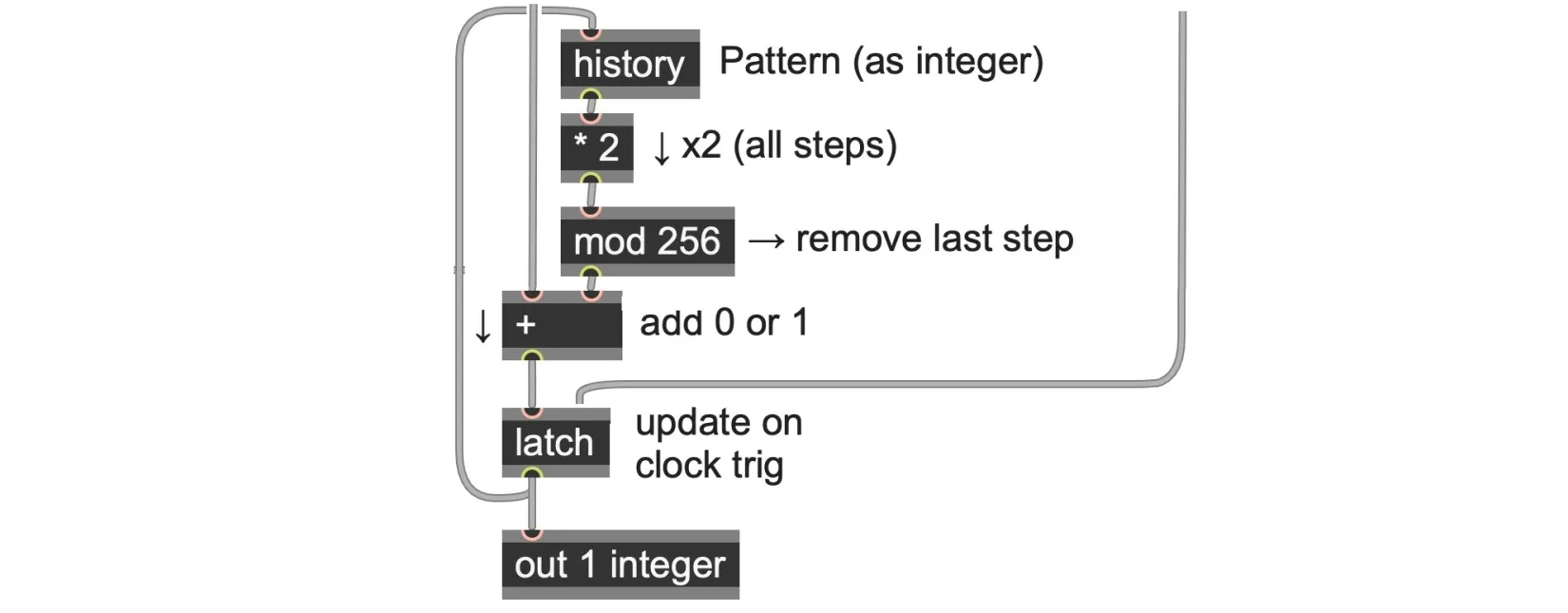
Here is what that means: For each clock trigger, we double the currently stored integer (equivalent to shifting the entire binary pattern right by 1 step); then add the new input (which is either zero or one), and then remove any surplus bits beyond stage 8 by using a mod operator to bring the integer value back into the 0 to 255 range.

Here is that circuit with an input source and clock added:

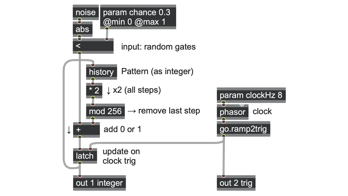
This isn’t merely simpler to patch — it’s more efficient, uses less memory, and is more flexible. For example, you can change the length of the loop simply by setting the value the mod operator uses to a different power of 2. To calculate what power of 2 you need for a specific pattern length (number of bits), you can use the exp2 operator.

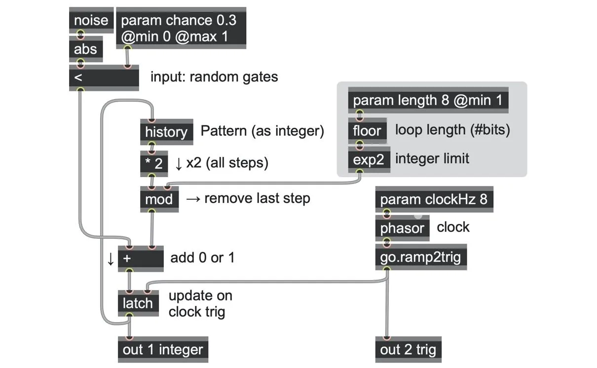
If the number of bits changes, this will also change how large the integer output can be. We could, however, normalize the output to a 0.0 to 1.0 range simply by dividing it by the limit value that the exp2 operator computed for us.

We can also get the value of the last step just by testing whether the result of the * 2 operator is greater than or equal to this limit value and use this “overflow bit” to feed the looping xor operator circuit like before.

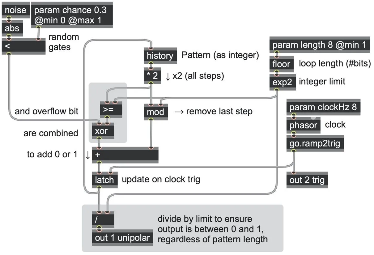
shift-register-integer.maxpat

Working with the bits of an integer

Shifting the bits one step to the right is far from the only thing we can do. Let’s look at a few different operations we can apply to the integer and what they may be useful for.

Extracting the first bit: If you want to read off the first bit from any integer, all you have to do is get the modulo remainder by 2, using a mod 2 operator. (Incidentally, this is also how we detect whether an integer is odd.)

Extracting all the bits: Perhaps we want all the individual stages to route into a mixer or to drive rhythmic elements. To pull out the 2nd bit, we can first shift the integer left one bit and then read off the first bit. We already saw that shifting right is like multiplying by two; shifting left is just the opposite, dividing by two. However, this can result in something that isn’t an integer (e.g., 3/2 = 1.5). We can fix that back into an integer by passing the result through a floor operator to remove the fractional part, resulting in 1.

So, to break apart an integer into eight bits, then one way to do it is to shift left by one bit progressively (dividing by two and throwing away the fraction via the floor operator) and using a mod 2 operator to extract the first bit of each.

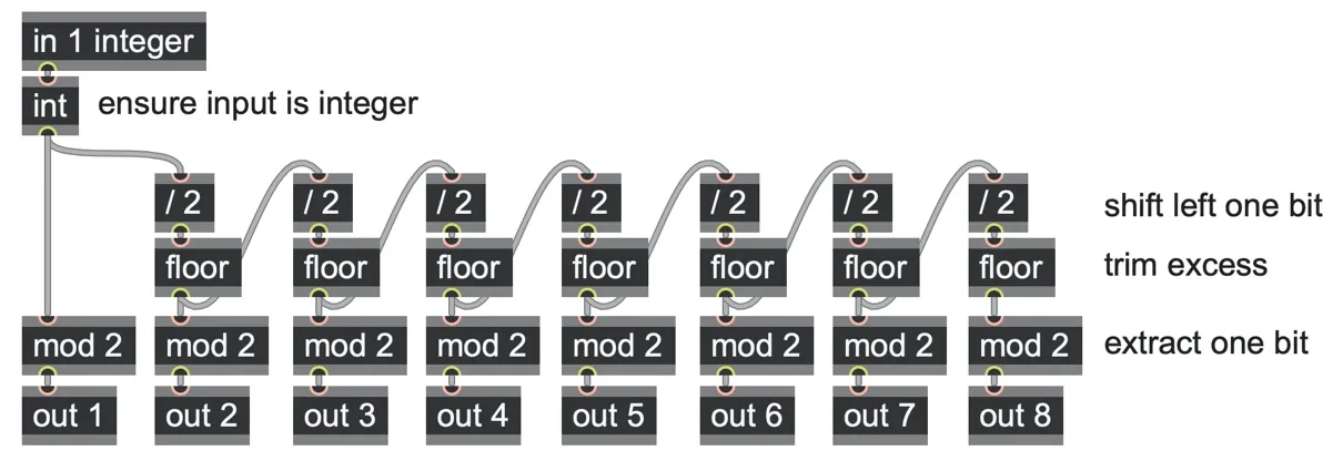
go.bit.unpack8.gendsp

Shifting N steps left or right: If you just want to right or left shift an integer by several steps, you can do it simply by multiplying by the corresponding power of 2. The effect of shifting N bits to the right is like multiplying by 2N, and shifting N bits to the left is like multiplying by 2-N, which is to say, dividing by 2N. Again, we add a floor operator to ensure the result is still an integer.

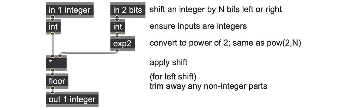
go.bit.shift.gendsp

A left shift can be used to reduce the bit depth of a sequence, as the left edge is trimmed away by the floor operator.

Limiting the total bits: We can also limit the bit depth of any integer just by trimming off the right end by removing any value greater than a certain limit using a wrap operator. For example, if we trim our number to 3 bits, then the limit is exp2(3) = 23 = 8. That means we can represent any integer from 0 to 7 with only 3 bits, so a wrap operator with the upper bound of 8 does the job perfectly.

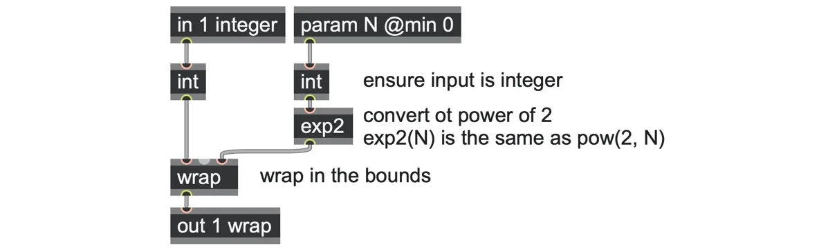
go.bit.wrap.gendsp

Extracting a subset of bits: We can combine these two operations to extract any subsequence of bits from an integer.

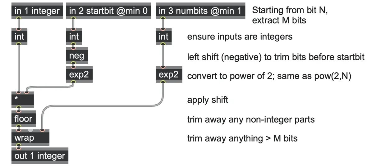
go.bit.extract.gendsp

If we are looking for a semitone pitch sequence, an 8-bit range of 0-255 is far too wide, but we could certainly work with smaller ranges simply by deriving our note values from a subsequence of fewer bits. Many of the hardware modules we mentioned earlier derive signals from just three bits in the register, which reduces the range to 8 distinct values since 23 = 8. For example, that might work well to select from 8 values of a pre-defined pitch scale or to choose between 8 sub-slices of an audio file. Using the go.bit.extract abstraction, we could even pick out several different 3-bit subsequences from the same integer.

Rotating a bit sequence: Bit rotation is similar to shifting but without losing any information. Any bits shifted off the left end appear at the right, and vice versa. That is, bitwise rotation is another kind of modular arithmetic: shifting the bits around is a movement in a cyclic space. You just need to define our bit depth in order to know where the right-side end is. If you look carefully, you can see this is just another combination of a left shift and a bit depth wrap.

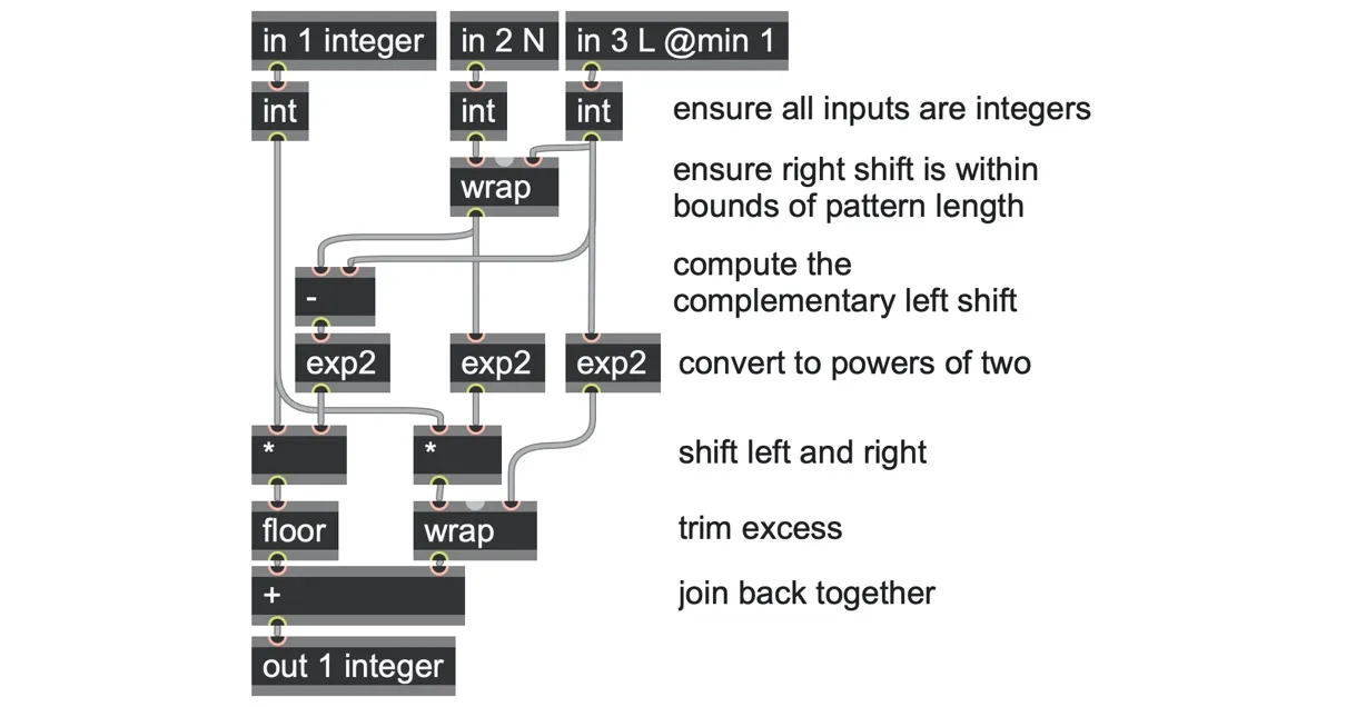
go.bit.rotate.gendsp

Understanding this operation opens up some amazing possibilities. You don’t have to limit yourself to always stepping the sequence one stage to the right in each clock trigger; you can have the sequence run backward or shift in larger steps just by choosing the appropriate bit rotation and then replacing the very first bit with the new input to your sequence.

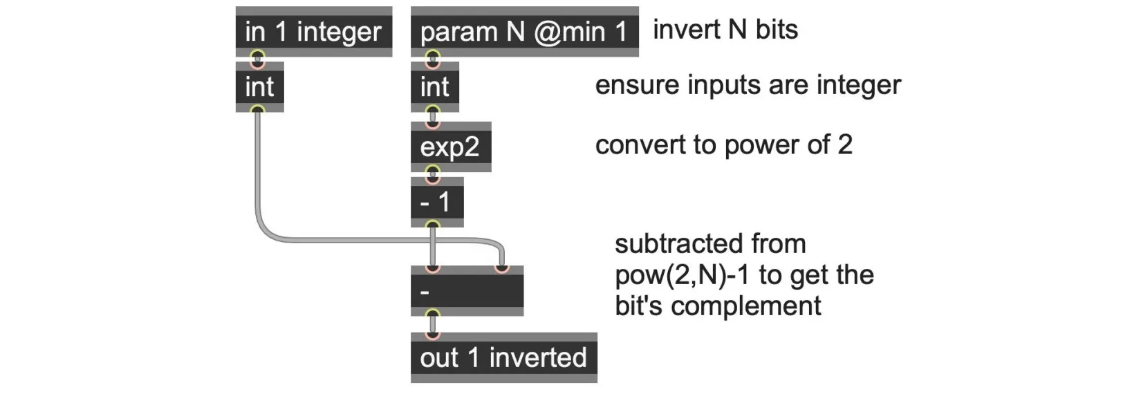
Inverting a bit sequence: We can also flip all the bits of an integer at once–so all the 1’s become 0’s and vice versa. If the integer has N bits, then the maximum value would be 2N-1, and we can subtract from that maximum to get our inverted output.

Taking this further: Combining a few of these bit operations, we can derive a wide range of related patterns. If you’re familiar with serial composition and musical forms such as fugue, those techniques may spark some ideas for you. Additionally, since the entire state of the shift register we’ve been looking at is expressed as a single integer, we can easily store many different patterns and recall them again later using a data or buffer operator. We can also generate entire new patterns at once with a go.random abstraction. That means we can undo changes to a sequence we don’t like, and we could explore mutations and crossovers for evolution between different stored sequences, for example.

Throughout this section, we have used a clock signal at a steady tempo to drive the shift register. However, this clock signal could also be replaced by a more patterned rhythm or something even more irregular. Let’s have a look at patterned rhythms next!

Euclidean rhythms (digitized ratios)

In Chapter 2, we looked at metric musical time as a cyclic phenomenon, which we represented as unipolar ramps, and we explored ways of producing more interesting rhythms using modular arithmetic. Another example of modular arithmetic at work in rhythm is Euclid’s algorithm for computing the greatest common divisor (GCD) of two whole numbers.

In 2004, Godfried Toussaint discovered that this method also happens to correspond to traditional rhythmic patterns of many musical cultures across the globe. In this rhythmic application, Euclid’s algorithm effectively spaces a number of events as evenly as possible over a given duration of a fixed meter.

All of these rhythms can be specified by just three integers:

• N = pattern duration, in beats (the dividend)

• K = number of events (the divisor)

• S = offset where the first event starts (rotation)

Euclid’s algorithm is a recursive procedure that requires a varying number of steps to be taken to compute the final pattern. This computation is also “outside of time” in the sense that it must generate the whole pattern at once rather than computing each step as needed. These factors make the algorithm itself less attractive for an "in-time" progressive computational context such as gen~.

We could write the Euclidean GCD algorithm using a codebox for() loop to implement the recursive operations, but there’s a much simpler way of getting the same results. It’s known as Bresenham’s line algorithm, which has been widely used in computer graphics for calculating the rasterization of a line onto a grid of pixels. This also happens to result in the most balanced way of spacing transitions over a fixed distance. Not only is this computable without recursion, it’s also “random-access”–you don’t need to compute the entire pattern all at once just to get the value at a single point.

Here is an example that spaces 7 events across 16 spaces:

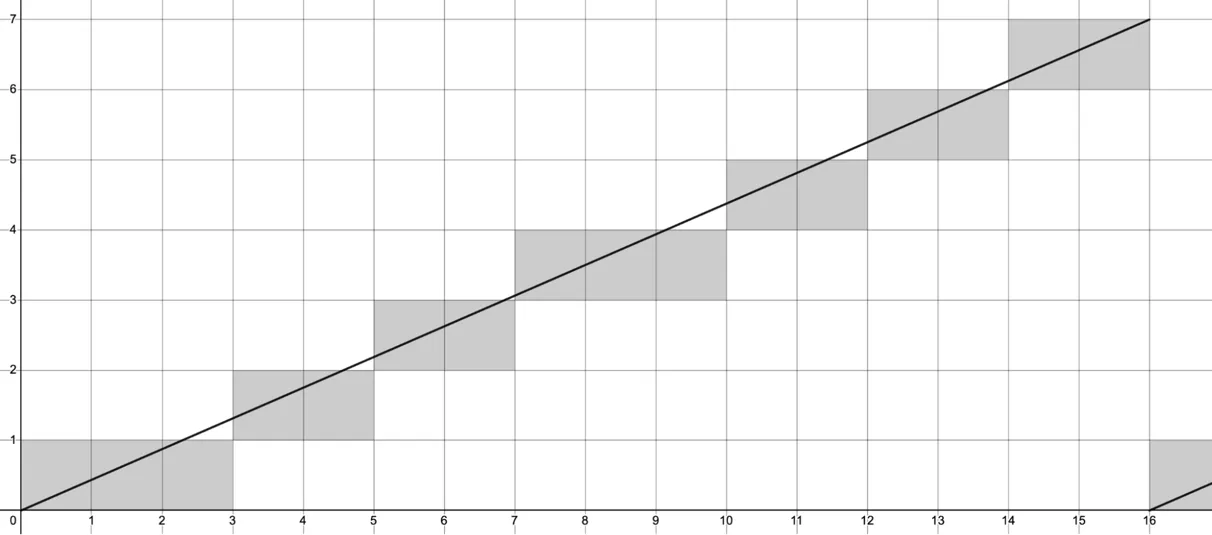
If we imagine a point walking from the start of the line to the end at a constant horizontal speed, we can make a few observations:

• Every column it passes represents one beat of the tempo. When it gets to the end of the line, it starts again at the beginning. So the number of columns (and the number of shaded pixels) is the loop length N=16, in beats.

• A cell is shaded if the line crosses the starting boundary of that cell. If we round the time down to the nearest integer column and round the height down to the nearest integer row, it will give us the shaded cell index.

• Every time the shaded cell moves up from one pixel row to another, we will trigger a sound event. So, the height of the line represents the number of sound events K=7.

• These two values determine the slope of the line as height/width or K/N taken together, which gives us the average rate of events.

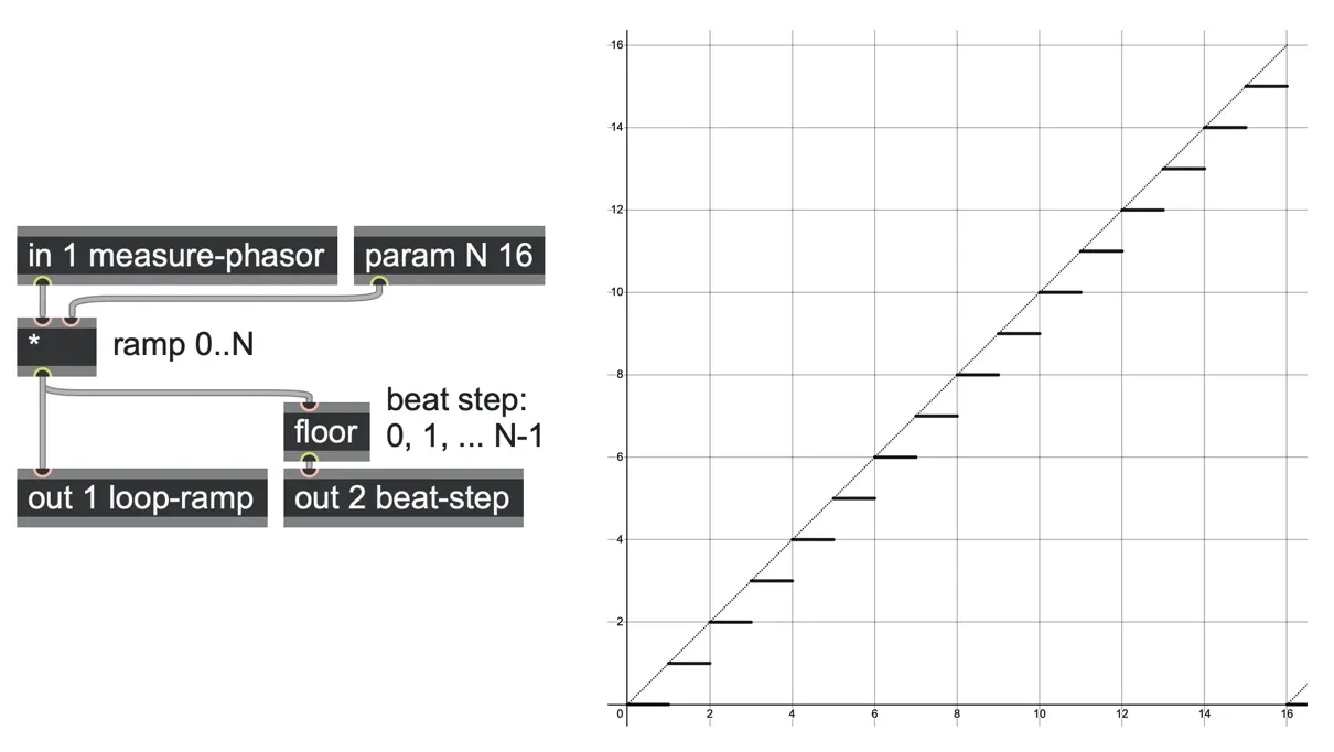
To implement this we’ll start with a step function aligned to the beat that counts from 0 to N. We can take a looping phasor, such as the ramp-per-measure produced by a go.ramp.frombpm abstraction, and simply multiply it by N (shown as a dotted line in the following graph), and then apply a floor operator to get the position of this line at the start of each beat (shown as a solid line in the following graph).

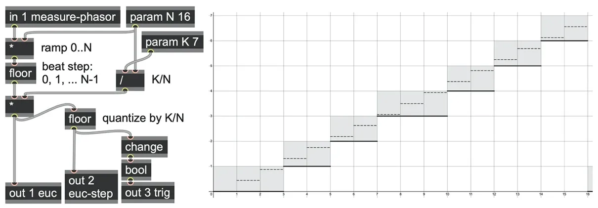
Next, we can apply the required slope K/N to this step signal simply by multiplying by K/N (shown as a dashed line in the following graph) and round that down using the floor operator to get the step signal that identifies the shaded pixels (shown as a solid line in the following graph).

Euclidean Ramps

We can get Euclidean rhythm triggers from this step function by tracking when it changes using the change operator and getting positive-only triggers from that via the bool operator. But since we already saw in Chapter 2 how useful ramp-based rhythms can be, we’d like to make our Euclidean rhythm generator also produce ramps for each of the events. Then we could use it to drive any of the LFOs we created in Chapter 3 for Euclidean LFOs!

The first question is this: what do we need to do to our existing ramp to make it restart from zero at every new event? If we knew what beat the event starts on, it would be simple: just subtract that from the ramp! As it turns out, we can compute the start point of our quantized events simply by applying reverse transformations.

First, we must re-scale our event step pattern, which runs from 0 to K-1, back to the loop beat pattern, which runs from 0 to N-1. We can do that by dividing by K/N (dashed line in the following graph), but—as you can see—we may end up with some non-integer results. To fix that, we can apply a ceil operator to round to the nearest whole beat (shown as a solid line in the following graph). That gives us the start point of every event in beats, which we can subtract from the loop ramp to get a ramp per event (shown as a dotted line in the following graph).

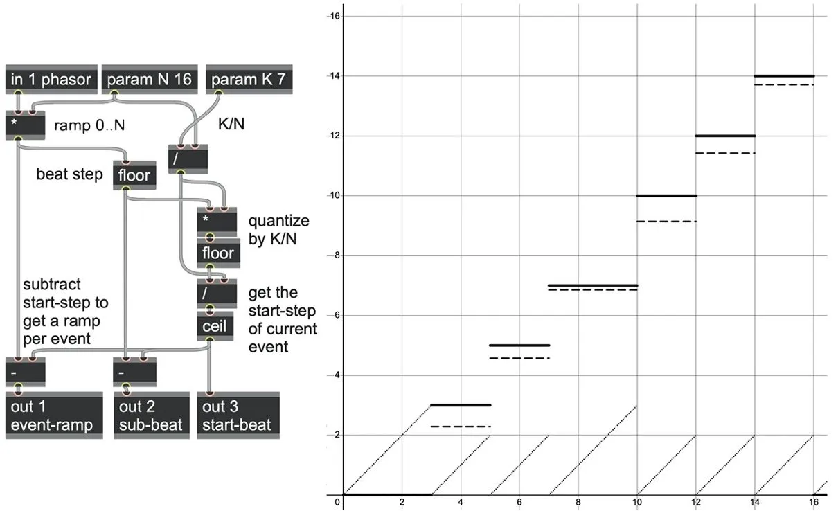
As you can see, these ramps are now aligned to the beats as we wanted, but unfortunately they are not normalized from 0.0 to 1.0 and thus may cause unwanted results with further ramp-based rhythm processing.

We could fix this if we knew not only when an event starts but also how long it will last (shown as a dotted line in the following graph), since dividing the ramp by this length would normalize the ramps (shown as a solid line below):

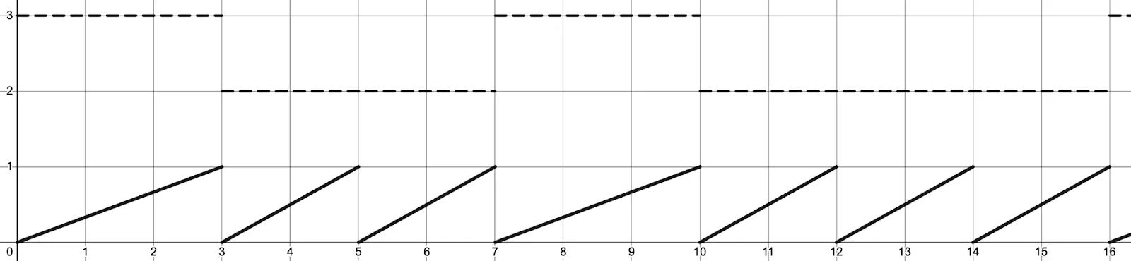
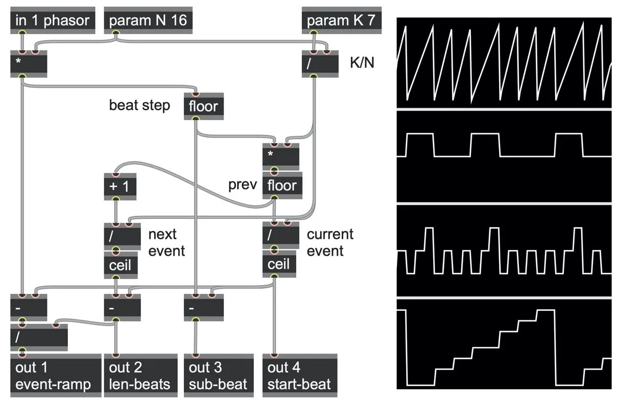
We can get the length of each event if we know when the subsequent event will happen, and computing their difference. To get the subsequent event, we can simply add one to our current position and apply the same division and ceil operations to compute the end point in beats. Then we can subtract the start and end points to get the length and divide by this to normalize the ramp:

We are still missing the parameter S for setting the offset of the Euclidean pattern. This is easy to add: first subtract the offset S from the incoming ramp, then wrap back into the desired range of 0 to N. While we are refining this patch, let’s also add some parameter handling, including using latch operators to sync our parameters to the beat and inserting floor operators to ensure the K, N, and S parameters are integers.

We might also want to work with polymetric loop lengths while still keeping our events on a constant tempo, which we could do in the same way as we did with the ramp.modulo.rhythm.maxpat patch in Chapter 2: by first multiplying by a beat division param beats, and then wrapping by our pattern length N.

Here’s what all these additions look like:

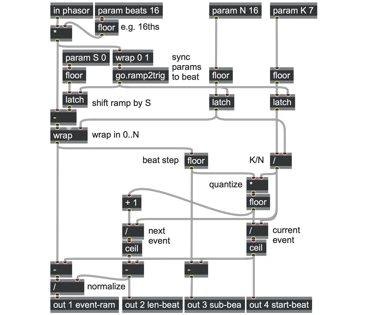
euclidean_rhythms.maxpat

Refinements

This is already a very useful Euclidean pattern generator, but we could think about extending some of the parameter handling further to make this patch more expressive. For example, we could extend the algorithm to handle negative values of K or N to run a pattern in reverse. This is actually quite simple:

• We use the sign operator to detect if K/N is negative and multiply our ramp by this sign accordingly.

• We use an abs operator after K/N for all other uses of it in the patch.

The euclidean_rhythms.maxpat patch shows an example of this.

Additionally, since the basic idea is to distribute a number of events (K) over a number of steps (N), then you would ordinarily expect K to be equal to or less than N. But that means that a “K” knob will have a certain range of travel (when K is greater than N) in which it doesn’t do anything useful. Wouldn’t it be more interesting to give the case where K > N a more meaningful or useful behavior? Here are some ideas:

• We could swap the values for K and N. So, for example, if N=4 and K=5, it would swap to K=4 and N=5, which is to say, we let N=max(K,N) and K=min(K, N). This is what the go.ramp.euclidean abstraction does.

• We could apply a wrap or fold operation to K by N. So, if N=4 and K=5, then K would be changed to 1 (via wrap 0 N) or to 3 (via fold 0 N).

• We could normalize our number of events in the range 0.0 to 1.0 as a “density” parameter and multiply this by N, and then round to the nearest integer to get the integer K value.

• We could ratchet (double-up) our steps. So, if N=4 and K=5, then every step would have an event, but one of those steps would have two events. First, we need to compute the required ratchet level R as the ceil of K/N, and then we use that number of steps to look ahead for our “next event” to compare with for the event length. Second, we determine the ratchet depth as exp2(R-1) so that we get double hits, then quadruple hits, etc., as R is 2, 3, and so on. The euclidean_ratchets.maxpat patch shows an example of this.

Once you get the hang of seeing the Euclidean rhythm generator as the rasterization of a straight line, another next step seems obvious: What if the line wasn’t straight? As we saw in Chapter 3, we can warp a timing ramp to produce all kinds of different shuffles and swings. Warps and changes like these will also propagate through our Euclidean ramp generator perfectly—but so will more extreme shapings of ramps.

You could even run one Euclidean generator into another. For an example, see the euclidean_LFO.maxpat patch.

Pitch spaces

Modular arithmetic shows up in music in other places besides metric rhythms. In most musical traditions, pitch is also cyclic: a particular set of intervals (such as the pitch classes of A, B, C, etc. of a Western classical scale), is a kind of step pattern that repeats over each octave. So, we might expect to be able to apply similar kinds of step and ramp processing to pitch signals too. But before we dive into that, we should look at how we can represent pitch as a signal.

An octave is the interval between the first and second harmonic of an overtone series, which means the interval over which a frequency is multiplied by two. That means the frequency difference between octaves is larger at higher frequencies and smaller at lower frequencies. However, that’s not usually how it seems to us as we hear it. As an instrument runs up through octaves, the distance between each subsequent octave sounds about the same. That is to say, we tend to hear octaves and other pitch intervals as steps of addition, not multiplication.

So, an octave is exponential in terms of frequency but can be seen as linear in terms of pitch.[46] Although most of our oscillators, filters, and so on are naturally parameterized by the exponential space of frequencies, there are a lot of musical advantages to working in a linear space of pitch. For example, pitch transpositions, chord inversions, and so on are all just simple additions and subtractions of numbers, no matter whether at low or high frequencies. And, as we shall see, working in linear scales of pitch can make quantization to scales very simple. For these reasons, we’re going to look at working in a pitch space rather than frequency space.

There are several conventions for pitch space in use in software and hardware synthesizers. For example, the MIDI protocol borrows from the piano’s Western 12-tone equal temperament (12-TET) system system in which the distance between any octave as an addition of 12 equally sized pitch steps, called semitones. Adding one to a MIDI note number means going up by one semitone; adding 12 means going up by one octave. We can convert between frequencies and semitones in gen~ easily thanks to the mtof and ftom operators, which convert from MIDI note numbers to frequency (Hz) representations, and vice versa. Note that the mtof and ftom operators work with any numeric value, not just whole numbers, so they will handle continuous glides and microtonal pitches if you want.

Another convention, more common to hardware modular synthesizers, works with the octave as the primary unit. In the “volt-per-octave” (or v/oct for short) convention, adding 1 volt to a signal means raising the pitch by 1 octave. This has the advantage that the integer part of a signal carries the octave register, while the fractional part of a signal carries the position within an octave, and it is less bound to a Western tradition. We are not dealing with electrical signal voltages in gen~, so we will simply refer to this representation as “octave” signals. The software with this book includes abstractions to convert between octave-based signals and MIDI or Hz representations: go.octave2midi, go.midi2octave, go.octave2hz, and go.hz2octave.

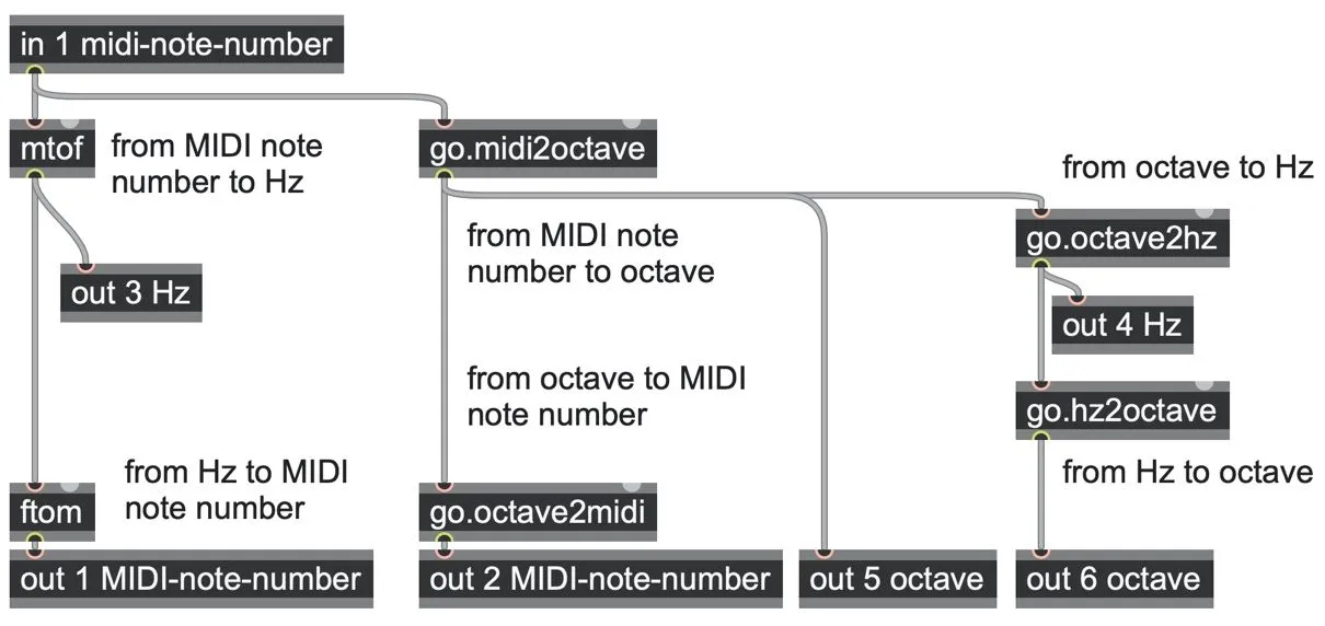
pitch.maxpat

(As an aside, we should note frequency can mean far more than pitch. For example, in Chapter 2 we saw how to express rhythmic frequencies in terms of beats per minute (BPM). We encounter the notion of a normalized frequency or "slope" (equal to a phasor's increment per sample) throughout this book, especially when creating oscillators.[47] We can also think about frequency in terms of its period, or the duration of one repetition, which is simply the reciprocal (!/ 1) of the frequency.[48] And for probabilistic processes frequency can mean a "chance per sample", where a frequency of 0.1 (e.g. as a parameter for a go.chance abstraction, see p. 96) means there is a 1 in 10 chance of an event firing on each sample, leading to an average density of 10%.)

Quantization

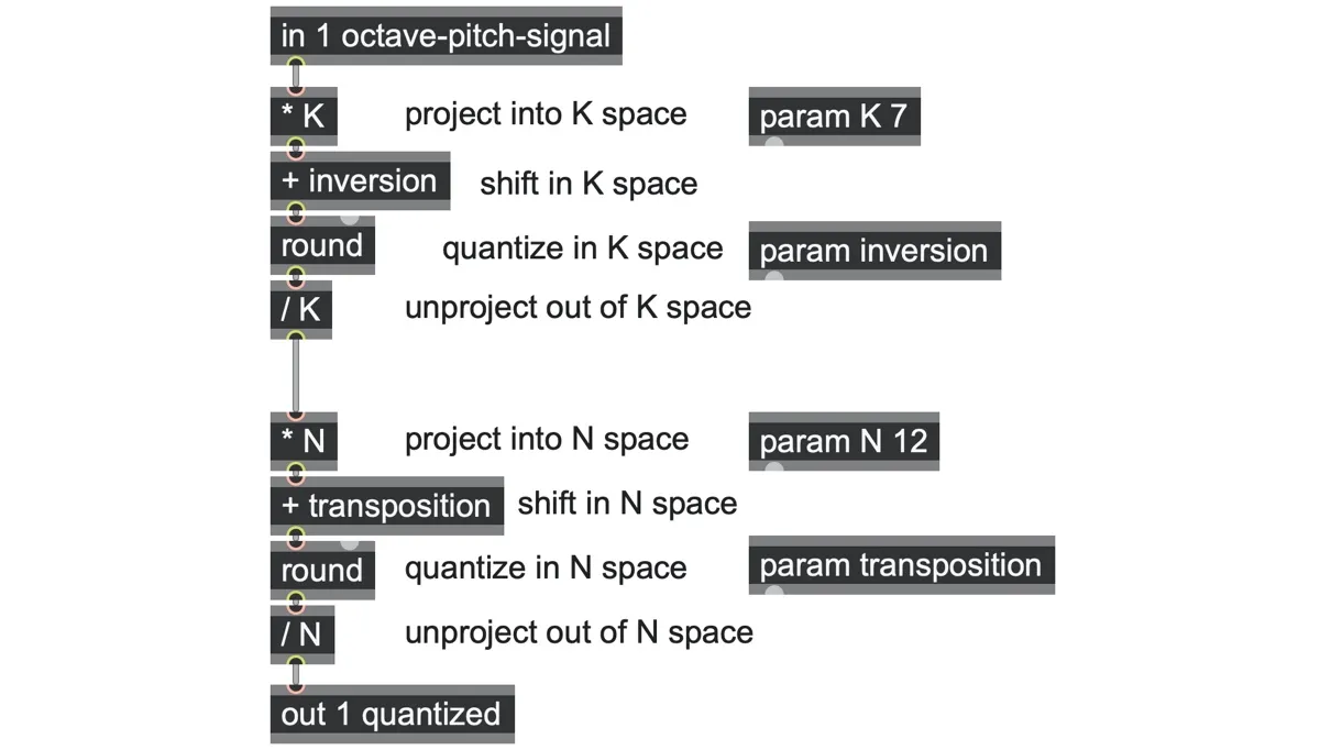
To quantize a MIDI note signal to the nearest 12-TET semitone, we can just round to the nearest whole number using a floor, ceil, or round operator. (Remember, the floor operator rounds down, the ceil operator rounds up, and the round operator rounds to the nearest whole number.) For an octave pitch signal, we can do the same, but we need to first project into a semitone space by multiplying by 12, where we can apply the rounding and then divide by 12 to return to our original octave-based pitch space.

If we wanted to apply a transposition or key change, we could simply add an integer bias while working in N-space.

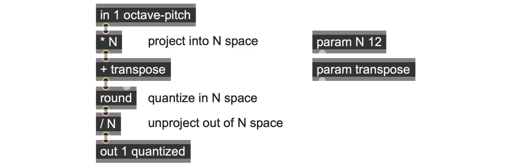
pitch-quantized.maxpat

This technique will work for any equal temperament base N, not just 12-tone equal temperament.

Euclidean patterns of length 12 produce common scales

Here is where things get interesting: if you quantize to one domain first (we’ll call it K), and then to another finer domain (which we’ll call N, where N is greater than K), you achieve exactly the same result as if you’d rasterized to the grid of KxN. Just as with the Euclidean rhythms, this quantization will align exactly to a grid of length N and will distribute K points as evenly as it can across it.

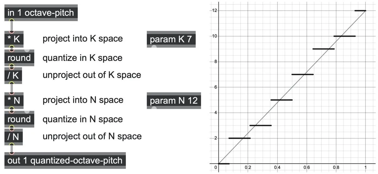
Remarkably, the same Euclidean rasterization algorithm we used before for rhythms can also be used to produce a variety of pitch scales common to many Western musical traditions. All you do is to set the number of divisions N to be equal to 12. In the Euclidean rhythms patch that corresponded to 12 beats per loop; in pitch space, it corresponds to the number of semitone pitches in an equal tempered octave. Here are a few of the distributions for different K values when N=12:

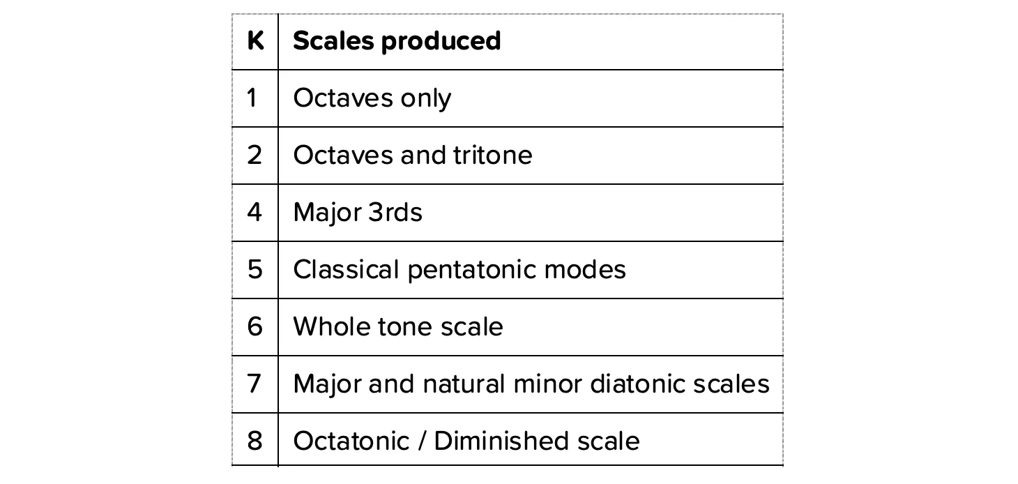
Moreover, where we can add an offset S to “rotate” the rhythm for Euclidean rhythms, here you can insert an addition in “N-space” here for key transpositions and in “K-space” for scale/chord inversions.

And if you can feed this patch with a ramp function or a triangle, you’ll get an arpeggiator.

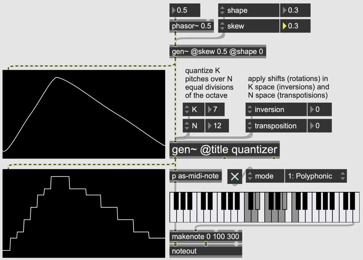
quantizing-pitch.maxpat

The space between notes

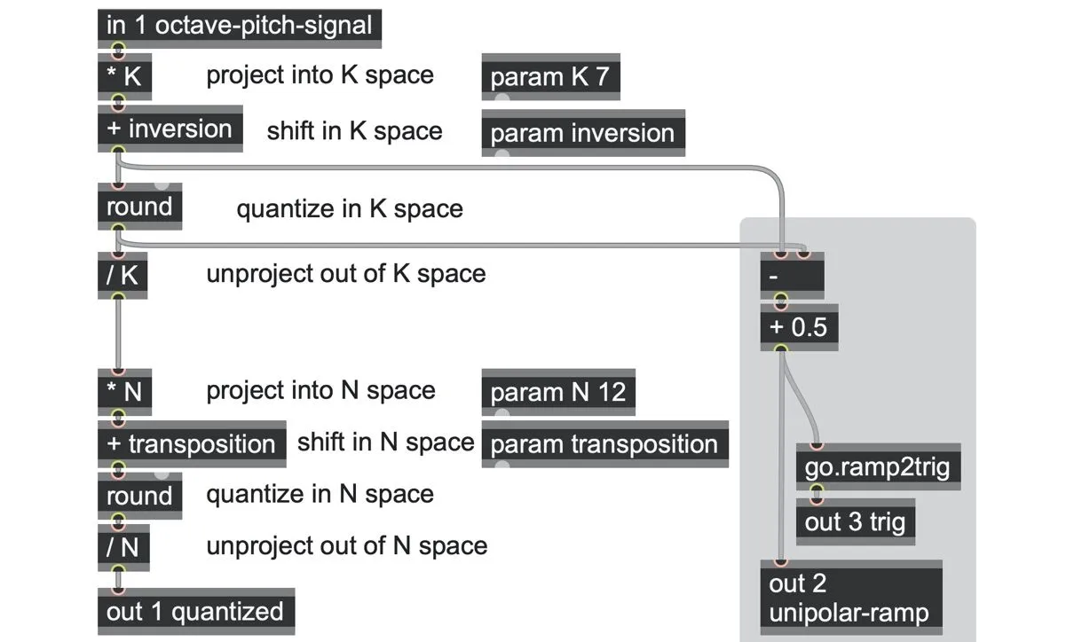
Some quantizers have useful trigger outputs to mark whenever the quantized pitch changes. We could do this by looking for a change in the output of the round operator, but—as usual—we think it is more interesting to output a unipolar ramp signal to tell you where you are between one note and the next, like this:

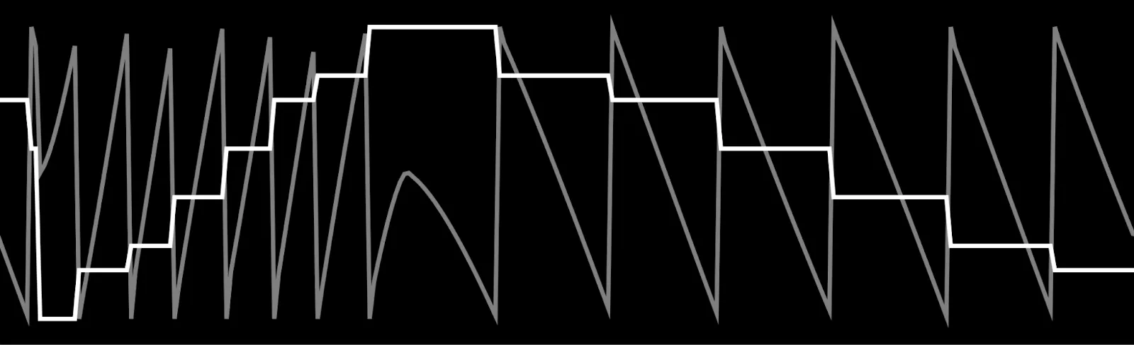
To do this, we can simply look at the difference (by subtraction) between the input and output of the round operator. That will begin at -0.5 as we enter a new note from below, and will rise to +0.5 just as we are about to leave the note from above. If we just add 0.5 to this difference, we will get a unipolar ramp running from 0.0 to 1.0 between each note as we rise (or from 1.0 to 0.0 as we fall).

quantizing-pitch.maxpat

We can derive triggers from this, as usual, using a go.ramp2trig abstraction, or apply any other kinds of ramp shaping we like.

Smooth-stepped quantization

A really useful variant of this is to soften the edges between each quantization step to create subtle glides rather than sudden leaps between notes. A neat way to do this is to crossfade between the quantized and unquantized versions of the input signal using a mix operator.

All we need to do to make the smooth glides is set the amount of crossfade applied according to how similar the quantized and unquantized pitches are. So, when they are similar, it snaps more to the quantized value; but when they are not as close, it blends more toward the original source pitch.[49]

The absdiff operator gives us a very simple measure of similarity (it subtracts the two inputs to get the difference, then tells you only the absolute magnitude, so the output is always positive). That difference will be 0.5 at most when the original signal is halfway between two quantized points, so we can multiply by 2 to get a range of 0.0 to 1.0 needed to drive the mix operator.

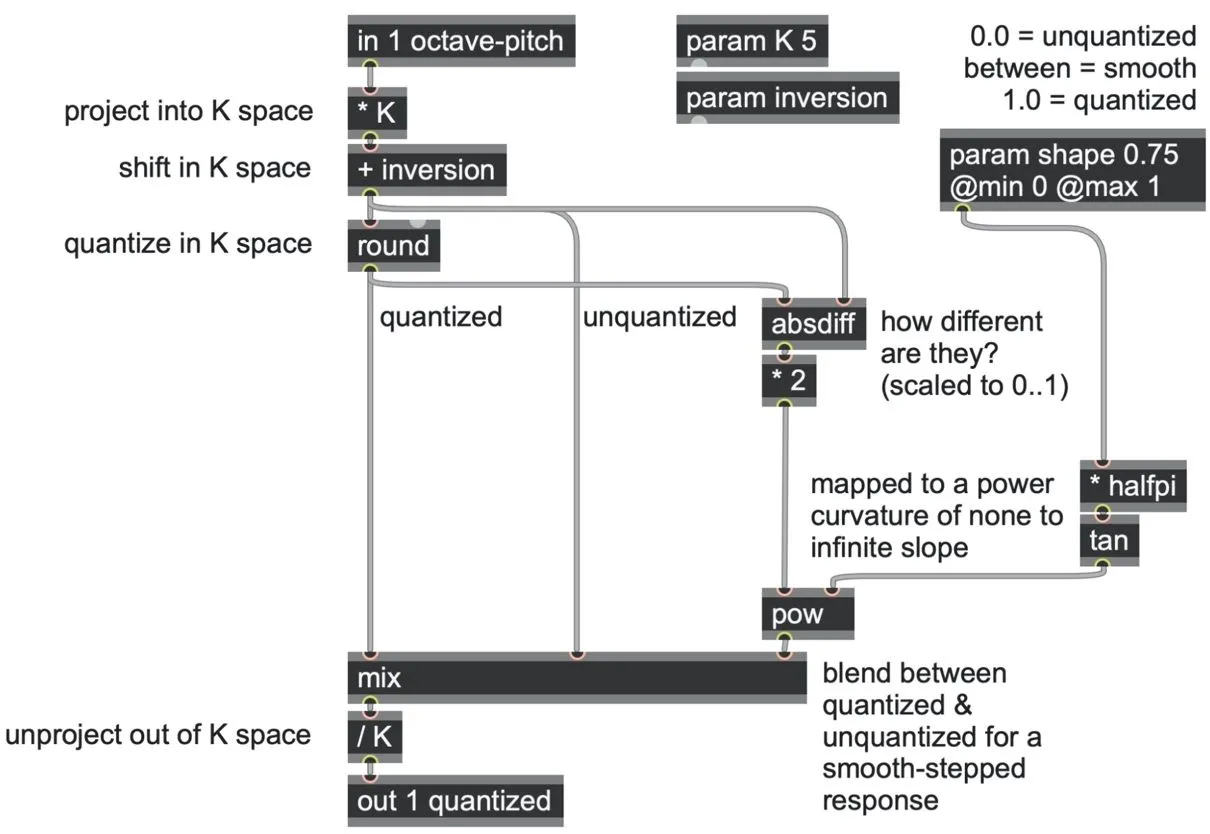
This effectively turns the sharp divisions between quantized levels into smoother glides. You might want to compare this to the pitch glides we encountered in Chapter 3.

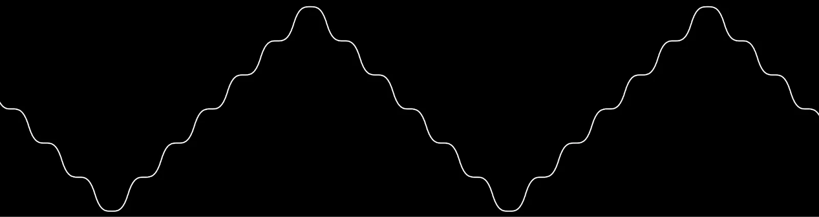
A smooth-quantized triangle wave.

The following patch is adapted for scale-based quantization with K and N.

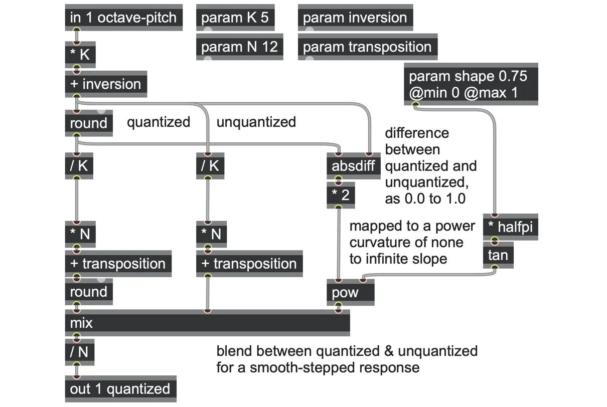
quantizing-pitch-smoothed.maxpat

Quantization as a timbral shaper

The sequence of operations of multiplying by N, rounding, and dividing by N is useful for any kind of quantization purposes, not just pitch! It is another example of the old trick of converting a problem into a more conducive domain where applying our desired changes is easier, and then converting back to our original domain. In fact, we already used this technique earlier in this book to convert tempo ramps to steps and generate random integers, for example.

It can also usefully process audio signals too. Quantizing audio produces a so-called “bitcrusher” effect, which transforms all curves into stepped waves. What’s interesting is that you aren’t limited to only quantizing to integer values; you can quantize to fractional steps, too (i.e., N can be a fractional number). This is important as it allows you to continuously vary N over time, which smoothly changes the depth of the bitcrushing effect to produce sounds that might remind you of pulse-width modulation (PWM), wave folding, or hard sync. Also, comparably to waveshaping, the results are very sensitive to signal levels: however with quantized bitcrushing, quieter sounds will be more intensely affected than louder ones.

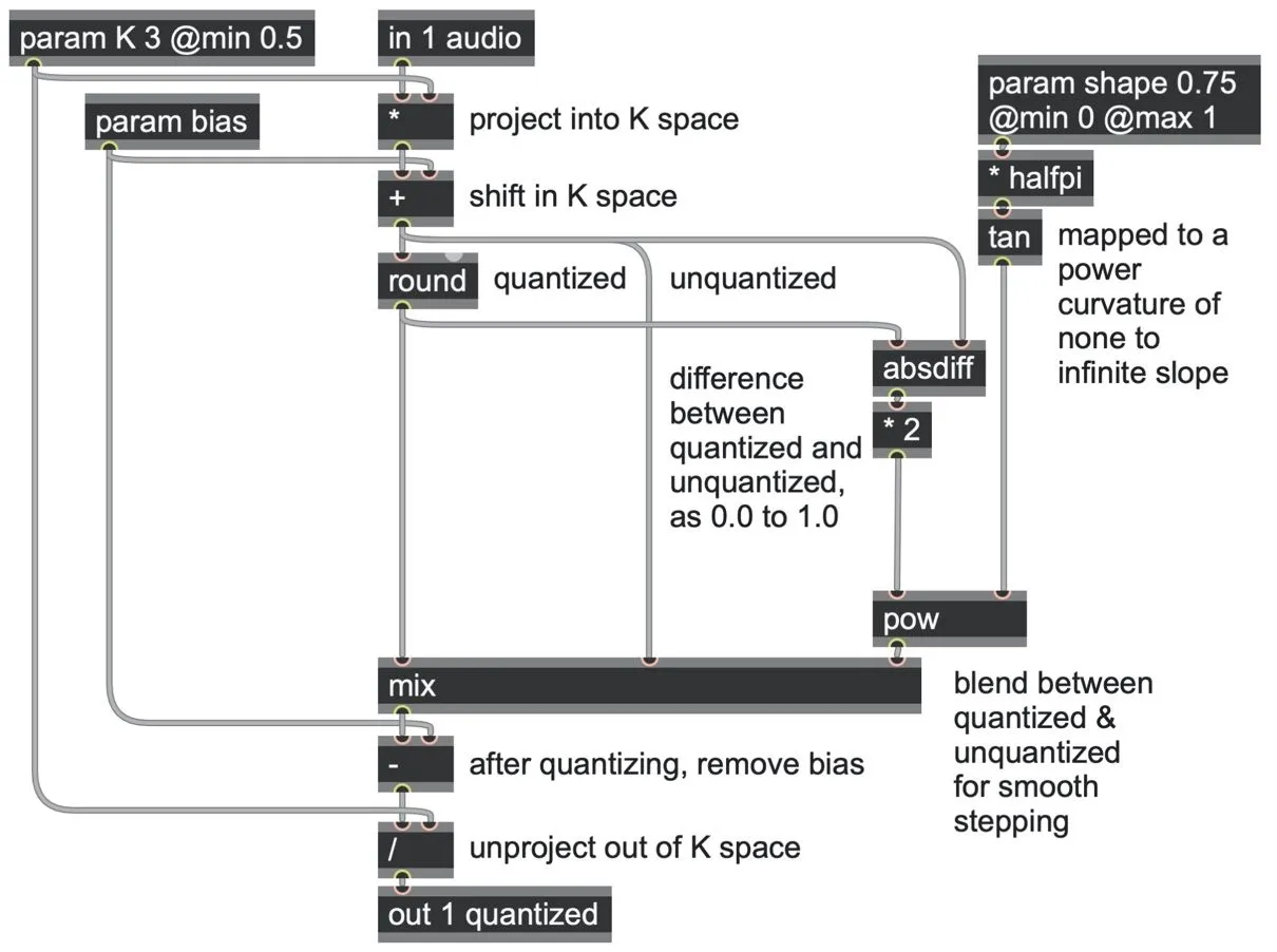
quantizing-audio-bitcrush.maxpat

In this patch, we incorporated the option of smoothing between the level changes, just as we did for the smoothed pitch quantizer. On audio, this acts as a crude lowpass filter and softens the harsher edges of the effect. You could try other unit shapers here too.

We also added the bias offset (just as we did for inversion/transposition in the pitch quantizer), but we are careful to reverse this bias after quantization to keep the audio centered around zero. The effect is more subtle at higher N, but with lower N adds another timbral aspect (reminiscent of wave folding asymmetry). Modulation recommended!

In fact, slight low frequency modulation of all parameters can be quite rewarding. Since this algorithm is very cheap, try mixing and panning a few together with slightly different parameters for a rich spatialized drone (for an example, see the quantizing-audio-bitcrush-drone.maxpat patch).