Chapter 9:
Navigating Waves of Data

In Chapter 2, we saw how to read and play a waveform stored in a buffer with a repeating phasor ramp by interpolated indexing using the sample operator. A phasor-driven sample patch like this is an example of a table-lookup oscillator, sometimes also called a wavetable oscillator:

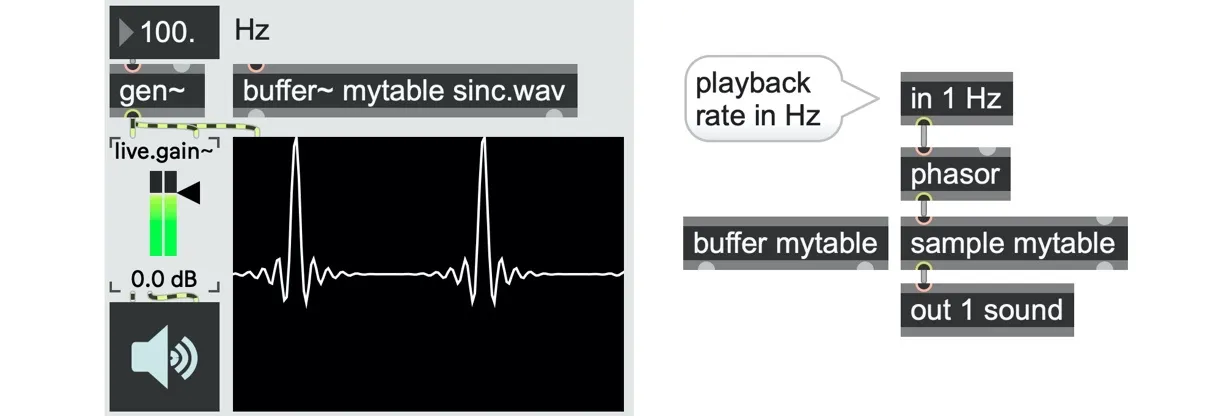
phasor_basic_table_oscillator.maxpat

The fundamental frequency of the oscillator is determined by the frequency of the phasor ramp itself, while the content of the buffer determines the actual shape (and thus timbre) of the oscillator. Since the buffer can have any combination of sample value data in it, the range of possible waveforms is practically infinite (although not all possibilities will necessarily sound interesting). Put another way, the phasor effectively navigates a data space that the buffer provides. In this chapter, we're going to look at a variety of different ways of organizing this data for greater variety, as well as a variety of different ways of navigating it.

Wavetables

The main drawback of a table-lookup oscillator, as in the patch above, is that the waveform's shape is always the same. It can feel sonically static and lifeless. If you wanted to switch between several different waveforms, you could have several other buffer~ objects and sample players, but that's not very efficient or flexible. Instead, the approach usually taken with wavetable oscillators is to pack several different single-cycle waveforms into subsections of a single buffer and dynamically switch (or blend) between which subsection of the waveform is playing at any time. For example, if our single cycle waveforms are each 1000 samples long, then we could store eight different single-cycle waveforms end-to-end as slices of a buffer of 8000 samples' length.

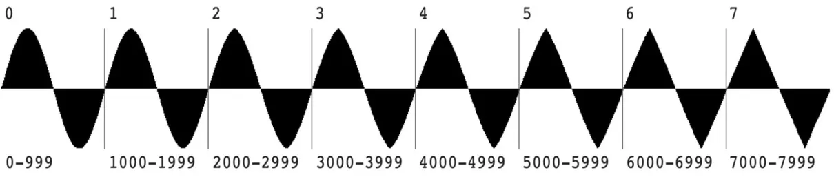
If we wanted to play the first waveform, we would need to loop over samples 0 to 999; if we wanted to play the second waveform, we would need to loop over samples 1000 to 1999; and so on. The wave operator is handy for that purpose. It takes a phasor signal at the first inlet to set the fundamental frequency and uses two additional inlets that specify the starting and ending sample positions of the sub-range of the buffer you want to play.[92]

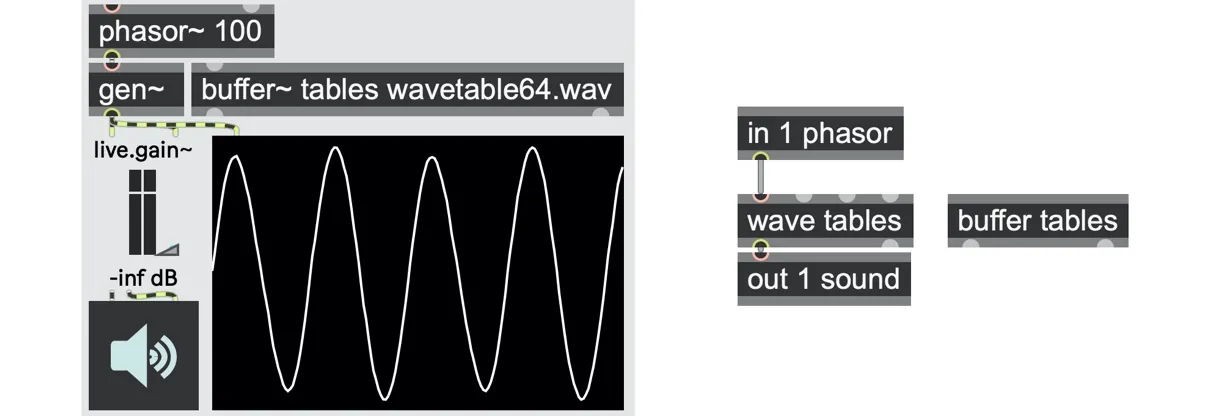
To build a wavetable player, we'll need a buffer~ containing several single-cycle waveforms. The software with this book includes a few example files, such as wavetable64.wav, which contains 64 individual waveforms. We can load that into our parent patch using a buffer~ tables wavetable64.wav object and reference this within a gen~ patch by adding a buffer tables operator. We can now read the data using a wave tables operator, driven by any unipolar ramp signal such as a phasor operator.

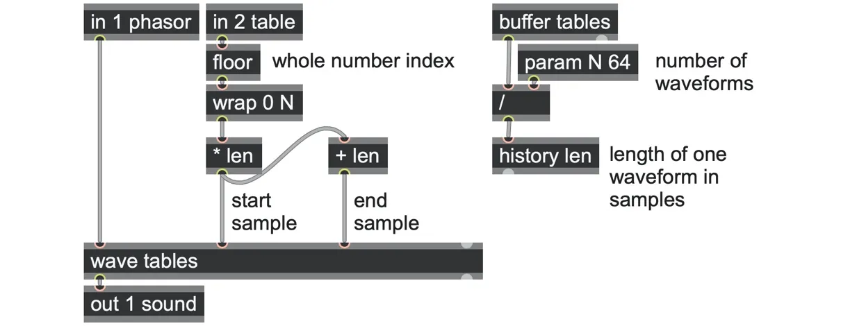
To pick out a specific waveform, we will need to set up the start and end sample indices of the wave operator. That means we need to know how many single-cycle waveforms the buffer contains, which we will provide using a param N 64 operator. We also need to know how many samples are in each of the single-cycle waveforms. Since the buffer operator broadcasts the total number of samples it contains from its first outlet, we just need to divide this by number of tables (param N) to get the sample length per table. It's handy to store this result in a named history operator, (such as "history len") so that we can re-use that name "len" throughout the patch, just like we can with param operator names.

We'll also need an input to select an individual table (in this case, from 0 to 63), which we can ensure is a whole number using a floor operator, and we can constrain that to the available range of tables using a wrap 0 N operator. Now our start sample index is simply this table number multiplied by the waveform length ("len"), and our end sample index is the start sample index plus the waveform length again.

Morphing between waveforms

Using the patch above we can switch between waveforms just by changing the signal value at in 2. However, as this value changes you might also hear clicks if the waveform changes abruptly from one shape to the next. Wouldn't it be better if we could smoothly blend (morph) between the waveforms rather than having these sudden switches? We can use a technique we have now seen many times in this book and which we will be using again and again in this chapter: to compute the two nearest whole number values (to select our two nearest waveforms) and output a linear crossfade or mix between them using a mix operator.

For this, we need an input that can support fractional indices that are part way between one waveform and the next, so the first thing we need to do is get rid of the floor operator after the in 2 table index input. To get the mix operator's crossfade factor, we can send the table index through a wrap 0 1 operator, representing our position between two whole number table indices. We can also subtract this fractional part from our table index to get the nearest whole number table index to the left and add 1 to that to get the next whole number table index to the right. These identify the two waveforms that we need to mix.

This is simpler than it might sound. For example, if our index is 2.3, then our two nearest waveforms are at index 2 and at index 3, with a crossfade factor of 0.3 between them, meaning we will get more contribution from waveform 2 than from waveform 3.

All we need is to repeat our wave operator twice, each working with one of the nearest table indices, and feed the results into the mix operator.

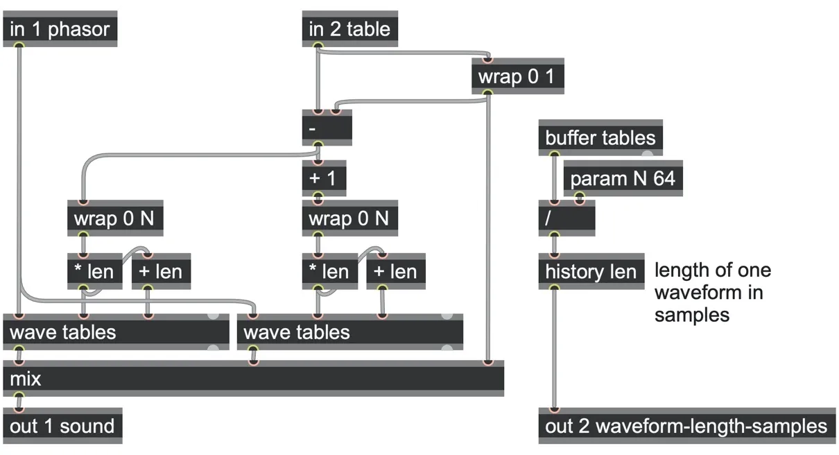
wavetable_1D.maxpat

Now we can plug in different kinds of modulation signals to the in 2 table input (such as an LFO multiplied by N) and hear smoothly morphing waveforms!

2D wavetables

With the previous patch, we can only morph left or right, through the set of waveforms in the buffer. Wouldn't it be nice to be able to morph in more directions? For example, if our set of 64 waveforms was arranged not in a flat sequence but instead in a two-dimensional grid of 8 columns of 8 rows, where each "cell" of the grid contains a single-cycle waveform, then we could morph left and right and also up and down across the grid.

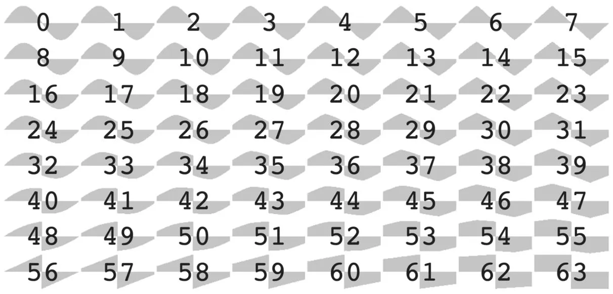
To select a cell within this grid of waveforms, we will need two index inputs—one to set our position across the columns (which we can call "X") and one for our position down the rows (which we can call "Y"). For a buffer containing 64 distinct waveforms in an 8x8 grid, there are eight possible indices per axis. So, now we will set our index range N to be 8, and we can compute the total number of waveforms as N2 or N*N, which we will need to figure out what our single cycle waveform length ("len") will be. Our patch starts like this:

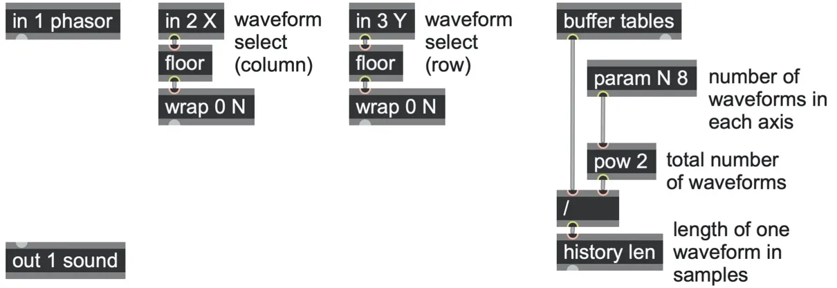
Notice that we used a floor operator to restrict X and Y to whole numbers for now (we'll add the blending back again later), and we added wrap 0 N operators to ensure they fit within the range of each axis of the 2D waveform grid.

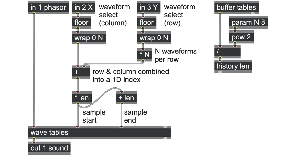
Even though we are pretending that the waveforms are laid out in a two-dimensional grid, they are still all in a linear series in the buffer. We will need a way to take a 2D grid position (such as column X=2, row Y=3) and convert it into a 1D index into the waveform series. We can figure out what the 1D index is just by taking into account the spacing. The first row starts at index 0, the second row at index 8, and so on, up to index 56 in the last row. So, we can simply take our row Y position and multiply that by N=8 and then add our column X position to get the 1D waveform index. For example, if X=2, Y=3, then the 1D index is 3*8+2 = 26.

Finally, to convert the 1D index into a sample start index for the wave operator, we can multiply it by the waveform length "len." The sample end index is always just the start index plus "len," just as we did before.

Morphing in 2D

Now, if we want to add waveform morphing, we can do it much as we did for the 1D wavetable. However, we now need to morph in two axes—blending vertically as well as horizontally over the waveform grid.

This means that we need to blend between the nearest four waveforms, which means we need four wave operators. For example, in the image below, X=2.8 and Y=3.9, which means blending between the four waveforms at indices 26, 27, 34, and 35 in the highlighted box.

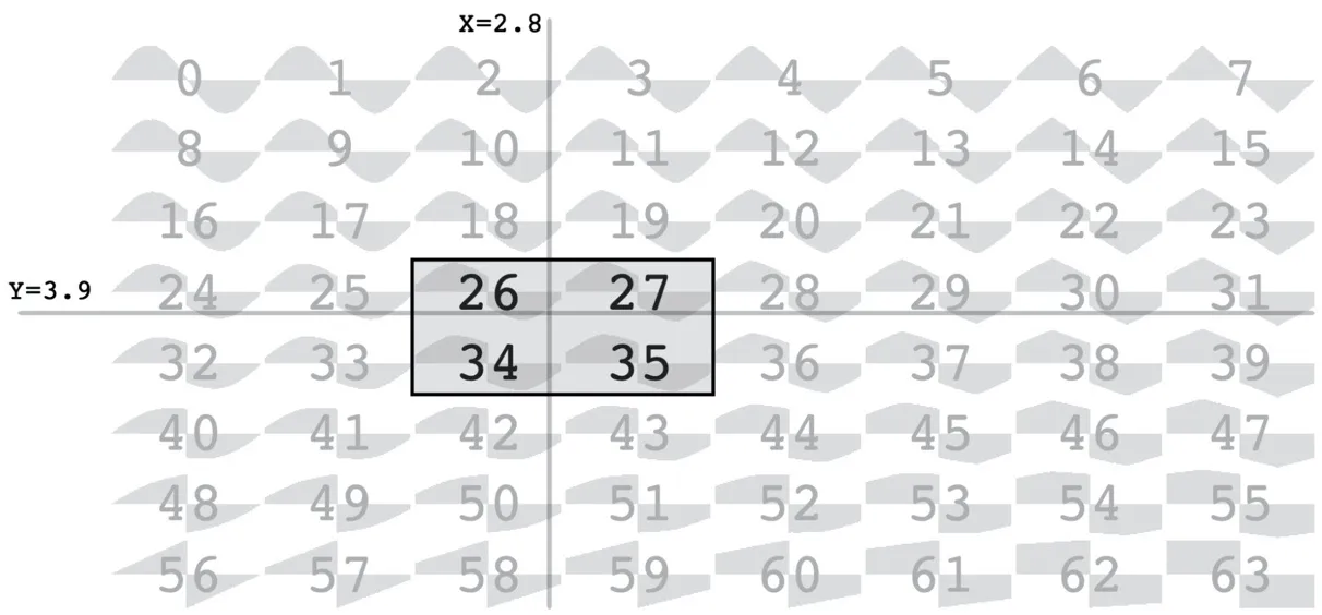
The output will be an appropriate linear mix of the four waves in the two axes, which is called "bilinear" interpolation. The overall structure might look something like the following patch.

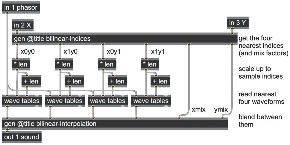
First, we feed the X and Y inputs into a bilinear-indices subpatch whose job is to work out the 1D index of the nearest four waveforms and also the horizontal and vertical crossfade factors that we will need. These 1D indices are converted into sample start and end positions for the four wave operators, whose results are fed into a bilinear-interpolation subpatch to do the actual crossfading.

Let's fill out those subpatches. For the X input, we'll do the same as we did before: capture the fractional component with a wrap 0 1 operator (which we also send out as a crossfade mix factor), subtract it from the X input to get the nearest column index to the left, and add 1 to get the nearest column index to the right. We added a wrap 0 N on each of these to ensure they are always in the valid range of columns. We do the same for the Y input, giving us the two nearest row indices above and below. Then, for each of the possible pairs of row and column indices, we can calculate the equivalent 1D index as before (using index = X + N*Y).

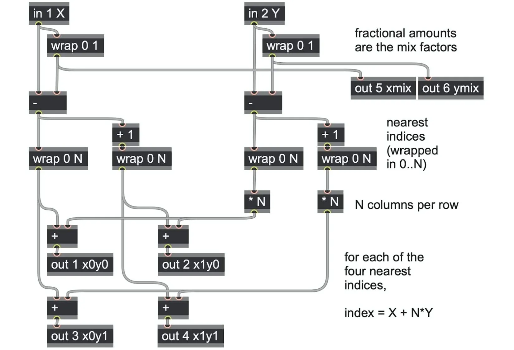
gen @title bilinear-indices

To perform the bilinear interpolation and blend between the four wave outputs in the bilinear-interpolation subpatch, we first apply blending in pairs across the X axis and then blend the results of these across the Y axis, using the corresponding "X mix" and "Y mix" factors accordingly. That is, we first blend across the rows and then blend the results across the columns. Even though we are blending between four waveforms, we only need three mix operators. That’s because the X axis was already mixed down before we came to process the Y axis.

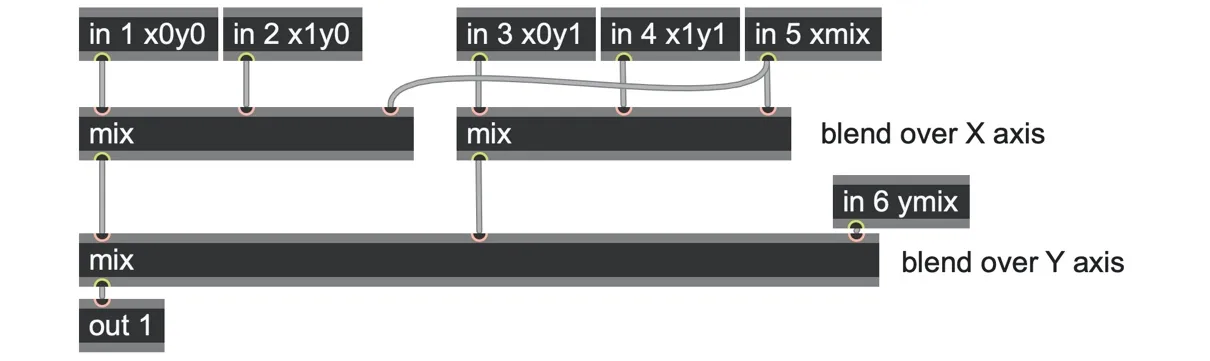
gen @title bilinear-interpolation

And with that, we can now smoothly wander all over the space of our 2D set of waveforms. This patch will respond pretty well already to some quite strong modulations: try plugging in a pair of LFOs for the X and Y inputs, or a pair of random walks, or one of the chaotic generators from Chapter 4, or indeed any pair of signals—we'll see more ideas for interesting orbits later in this chapter.

To make it a bit easier to try out different control signals, it would be handy if the X and Y inputs were expressed in a unipolar range, which we can do simply by multiplying unipolar inputs by N before feeding into the bilinear-indices subpatch.

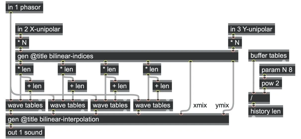
wavetables_2D.maxpat

3D wavetables

Now that we have seen how to extend from waveform selection over a 2D list into waveform selection over a 2D grid, we might have an idea how we could take this into waveform selection over a 3D volume!

First, we will need a file that represents a cubic volume of NxNxN waveforms. For example, the software with this book includes a wave file called 3x3x3.wav, which contains 27 single-cycle waveforms. Although they are stored in the wave file end to end in a linear arrangement, we can imagine those 27 single-cycle waveforms in a three-dimensional arrangement as a 3x3x3 cube, as in the following image:

Dividing a 3D parameter space into cells like this is similar to the idea of the voxel[93] used in computer graphics. Each of the waveforms stored in our buffer can be seen as a point in a regularly spaced 3D grid. That means that we'll need three parameters (X, Y, and Z, for horizontal, vertical, and depth) to pick out an individual waveform, each in a range between 0.0 and 3.0. Any trio of X, Y, and Z parameters (three values in a range of 0.0 to 3.0) will result in a unique waveform as its output.

The numbers in the cube image above are the order of the waveforms within the wave file, which is to say, their 1D index. As before, we'll need a way to convert from a 3D X, Y, and Z coordinate into one of these 1D indices. Looking at those numbers in the image above, you can see that if you are moving horizontally right across the cube increases the indices step in ones; moving vertically up increases in steps of three (to make space for the X coordinates), and moving in depth into the cube increases in steps of nine (to make space for X and Y coordinates). So, the 1D index can be computed from the trio of X, Y, and Z positions using index = X + N*Y + N*N*Z.

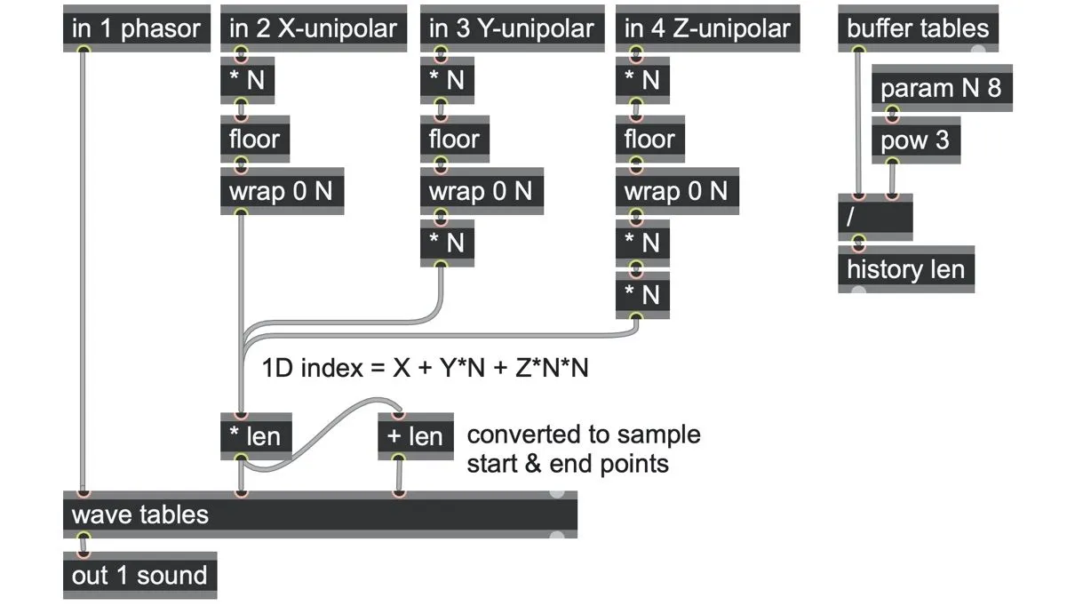
Here the number of tables is computed from the param N by raising to the power of 3 (cubing) using a pow 3 operator in order to compute the total number of tables, and from there the length (history len) of each waveform in samples.

Morphing in 3D

As before, the morphing "space" between each of the waveforms in this grid can be filled in by interpolating between them; but now we will need to interpolate between the eight nearest waveforms!

This means we will need eight wave operators and eight sets of indices for the nearest waveforms to our desired point. We'll also need a way to blend those eight nearest waveforms together smoothly as you modulate along any or all of the horizontal, vertical, or depth axes. This is called trilinear interpolation because it crossfades through three axes.

Here is what the outer structure of our patch looks like:

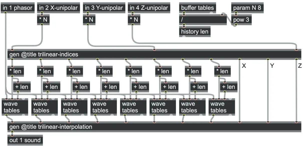
wavetable_3D.maxpat

The trilinear-interpolation subpatch replicates the same structure as the bilinear-interpolation patch, but now cascading the outputs of the eight wave operators through three layers of mix operators, one layer per axis. The first resolves the X axis, blending the eight waveforms into four; the next resolves the Y axis, blending these four into two, and the final stage blends these two along the Z axis, resolving into a single output signal that represents the 3D wavetable playback. Here is what that looks like:

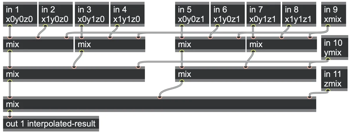
gen @title trilinear-interpolation

And as with the morphing 2D case, the trilinear-indices subpatch finds the nearest whole number indices in each axis, labeled in the following patch as x0 and x1, y0 and y1, and z0 and z1 (and the fractional parts are sent out of the patch for use by the trilinear interpolator).

Each of these indices is wrapped based on the number of waveforms per axis. Then, each possible pairing of these X, Y, and Z coordinates is passed through the function index = X + N*Y + N*N*Z to compute the corresponding 1D position of the waveform in the buffer. You might notice that the full set of permutations of combining the X, Y, and Z values follows a binary pattern.

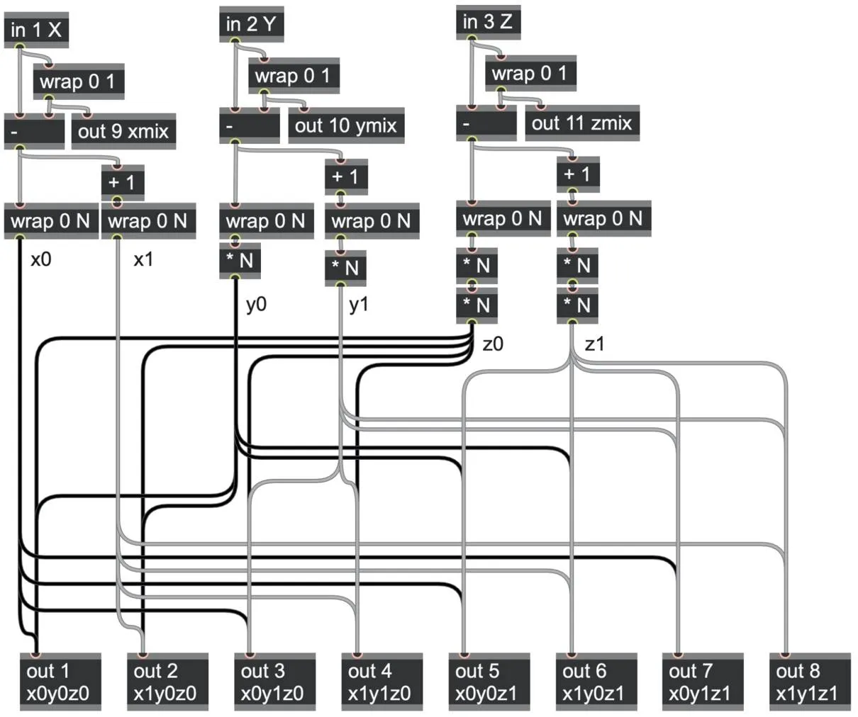
gen @title trilinear-indices

We now have a fully functioning, 3D morphing wavetable navigator! Since the number of waveforms per axis is set by a parameter, we could load a different set of waveforms (say, 4x4x4, or 8x8x8), and the only modification we need to make is updating the parameter N.

While we can explore the 3D wavetable by changing the X, Y, and Z inputs manually, this patch is tailor-made for modulation with signals at audio rates. The relations between the X, Y, and Z modulations will carve out different trajectories through the cube of waveforms. There are many ways we might consider doing this—perhaps, for example, using three phasor operators running at prime number rates for an aperiodic orbit.

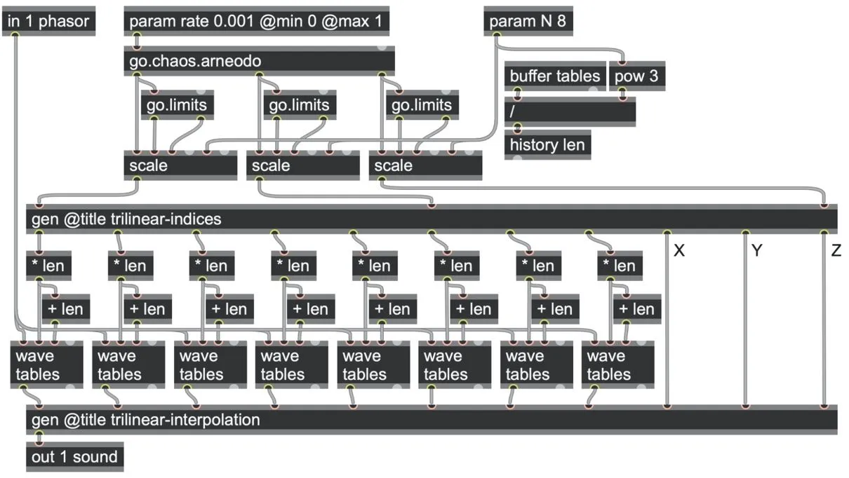
Alternatively, we could use one of the chaotic attractor patches from Chapter 4, most of which already output three related signals. All we need to do is to scale the attractor patch's three outputs to the input range that the 3D wavetable patch requires, which we do in the wavetable_3D_attractor.maxpat example using go.limits abstractions and scale operators.

Generating wavetables

The wavetable_3D_attractor.maxpat patch also shows how the 8x8x8.wav file itself was generated. We're providing this as an example of how you can generate wavetable data into a buffer procedurally using GenExpr code in a codebox.

In this patch, we generate the buffer one sample at a time so that the expensive computation it takes is spread over time. It only takes a few seconds to fill up the buffer, representing 8x8x8 = 512 waveforms of 1024 samples each. We work through the samples of the buffer using a cascade of counter operators. The first counter loops over the length of each waveform by means of the "len" argument. Its middle outlet outputs a trigger whenever it completes a lap, which is fed into the next counter operator. This one loops over N to account for each waveform in the X axis. Its lap trigger then cascades to another counter N for the Y axis, which cascades to a counter N for the Z axis. These four counts: the sample index "I" and the axis indices X, Y, and Z are fed into a codebox.

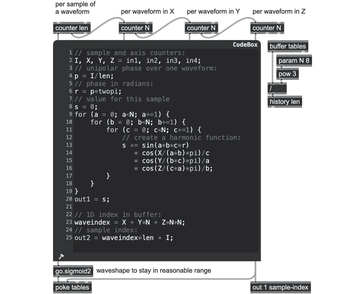
The outputs of the codebox are the sample value to write and the sample index to write it to, which feed into the corresponding inputs of a poke tables operator. We also sent the sample value through a go.sigmoid2 waveshaper abstraction to get more saturated dynamics across the wavetables.

The internals of the codebox come in three parts. First, we convert the waveform sample index into a unipolar phase over the waveform and then a phase in radians, which is more convenient for use with sin and cos operations.

Second, we compute a sum of NxNxN sinusoidal harmonics, each weighted differently according to our X, Y, and Z coordinate in the 3D cube. When N=8, this means we are computing 512 sinusoids per sample of the wavetable. (That's a pretty expensive calculation, which is why this is worth spreading over time and saving into a wave file rather than computing it on demand!)

Finally, we compute what the actual index of this waveform should be in the 1D list, using the same index = X + Y*N + Z*N*N expression we have used previously. Then, to convert that to a per-sample index, we multiply by "len" and add the sample index "I."

You can replace the inner code with whatever functions you prefer to use to fill your wavetables, of course—it's up to you! When you have generated a wavetable you like, send a "writewave" message to the buffer~ object in the parent patcher to save it to disk.

Band-limiting wavetables

So far, we've been reading from the buffer using sample or wave operators, Ih use linear interpolation to render a perceptually smooth output from what is actually a finite, discrete set of data samples. For some waveforms, that is good enough. But for other waveforms - particularly shapes with strong harmonic series such as saw and square waves - wavetables can introduce aliasing noise during playback, and linear interpolation alone won't prevent it. In this section, we'll look at why this noise appears and some strategies to address it.

First, why is interpolation needed at all? Since we can be playing the wavetable at many different rates (pitches), it is unlikely that the sample frames of real-time passing in the patch exactly line up with the sample points of the wavetable buffer. For example, if our wavetable is made of 64 samples, and our sampling rate is 48kHz (48000Hz), then the only frequency that they exactly line up is 48000/64 = 750Hz.

It looks like this:

In the image above, the horizontal steps represent the data in the wavetable (representing a sampled sine wave), aligned with a density of 1.0: one wavetable sample per sample frame of real time across the X axis.

If we play the wavetable oscillator slower than 750Hz, the wavetable samples will be stretched out; if we play higher than 750Hz, they will be compressed more tightly together than the sampling rate. We can call this the relative sample density. For example, at 150 Hz, the relative sample density is 0.2 (as there is only one wavetable sample for every five samples of real time):

For most oscillator frequencies, this means we will have to estimate what the wavetable's data should be at fractional points somewhere between the actual data samples of the wavetable. That's what we use interpolation algorithms for. If we didn't use interpolation, the playback would follow the stepped graph above, which would be much noisier (try using a wave tables @interp none operator if you want to hear what this sounds like).

By default, the sample and wave operators use linear interpolation to estimate the value at any fractional point by taking a weighted average of the two nearest sample frames in the buffer. This emulates a simple ramp between samples, as represented with a dotted line in the following graph:

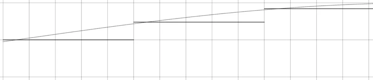
As you can see, linear interpolation does a reasonable job of filling in the gaps between wavetable samples, but it doesn't eliminate all of our noise problems. If we play through the buffer at a rate high enough that the relative sample density becomes large, so there are many wavetable samples per sample frame of real time, then we may end up trying to synthesize a signal that has more detail (higher frequency information) than can actually be rendered at the current sampling rate.

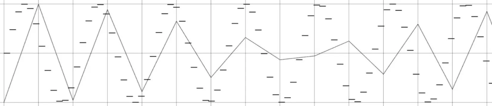
For example, in the graph above, the wavetable oscillator is playing at 5.9x the original frequency, with 5.9 wavetable samples for each passing sample frame of real time. This has far too much high frequency detail to render at the current sample rate. Notice that the interpolated output (the dotted line) no longer follows the original sine wave and even flips to be completely out-of-phase (upside down) part way through the graph. This inability to represent the detail, and the interference pattern that ensues from it, is an example of aliasing.

Note that this is not a limit of gen~, it is a fundamental property of any discretely sampled system. Whatever the sampling rate is, we cannot render any information that is more than half this sampling rate (the Nyquist limit). Nothing can appear to move faster than samplerate/2. The kind of aliasing that results from frequencies higher than the Nyquist limit is one of the most pernicious sources of undesirable noise in digital signal processing in general.

In the next chapter and moreso in book 2 we will be looking much more deeply into addressing the challenges of aliasing, but here we are going to work through strategies we can apply to wavetable playback. One of the first principles to know is that we can't filter out frequencies that have already aliased — we have to try to prevent those high frequencies from being generated in the first place (this is also called band limiting a signal). To address the problem with the wavetable playback, we want to avoid rendering a wavetable at a higher resolution than the current real-time sampling rate can support. We're going to do this using two strategies: a windowed-sinc interpolation filter and mipmapping.

Sinc interpolation

Let's start with sinc interpolation. We already saw in Chapter 6 that filtering and interpolation are very closely related. A linear interpolation or mix operation applies a weighted average, which will tend to smooth out differences (higher frequency detail) and preserve only the more similar, lower frequency parts of a signal. Another way of seeing this, which might not be as obvious, is that we are multiplying two samples of our wavetable by a two-sample triangle window and outputting the sum.

As we saw in Chapter 6, the linear interpolation of a mix operator means multiplying one sample by the unipolar factor "a" and the other sample by "1-a" and adding the results together. But here's yet another way to look at it: these two factors of "a" and "1-a" are simply intersections with the rising and falling edges of a two-sample triangle window! Imagine this triangle sliding across the data points of the buffer, always multiplying by the two nearest points that intersect with it and summing the result; this is exactly equivalent to linear interpolation.

Summing multiplied pairs of points like this is called convolution. Other kinds of interpolation, such as cubic, spline, etc., are also convolutions, but with different window shapes and usually summing more sample points. (We saw some of these when building smooth random signals in Chapter 4. The more points we use, the deeper the filtering can be; while the specific shape of the window determines the spectral distribution of the filter response. The filtering effect of linear interpolation spreads out widely over the frequency spectrum (decreasing by only -6dB per octave), which means it is not a good choice for suppressing aliasing noise. What we need is a filter that can attenuate high-frequency detail much more sharply without compromising the frequencies below.

Instead, we're going to convolve our wavetable with a windowed-sinc function, which can preserve energy well up to a certain point but soon silences frequencies above that point.

A sinc waveform can be generated using the mathematical function sin(x)/x, which has the characteristic rippled impulse shape in the image above. Since a pure sinc function is known to be bandlimited, then any convolution with it would also be bandlimited in the same way. Unfortunately however, the pure mathematical sinc function is infinitely long, and would need infinite sample points for convolution. Instead, we use a "windowed sinc" function, which simply means that the infinite sinc curve is tapered to zero after a certain number of ripples.

For our windowed-sinc wavetable patches we pre-calculated a sinc shape tapered using a Kaiser window for use with eight-point interpolation, which we stored in the go.sinc8.wav file in the software with this book. We can load this into our parent patch using a buffer~ sinc8 go.sinc8.wav object and reference it in gen~ using a buffer sinc8 operator.

Using an 8-point sinc interpolation means that we will need the eight nearest consecutive sample points from our wavetable, which we can read using eight peek operators. We're using peek here because we explicitly don't want any interpolation at this stage of the patch; we're doing the interpolation ourselves next.

Each one of these peek outputs will be multiplied by a corresponding sample from the sinc8 buffer. We are using phase offsets and sample operators for the window because interpolating the window does make sense. The crucial part is that we should shift these samples in time according to the fractional interpolation factor we computed earlier.

Put together, it looks like this:

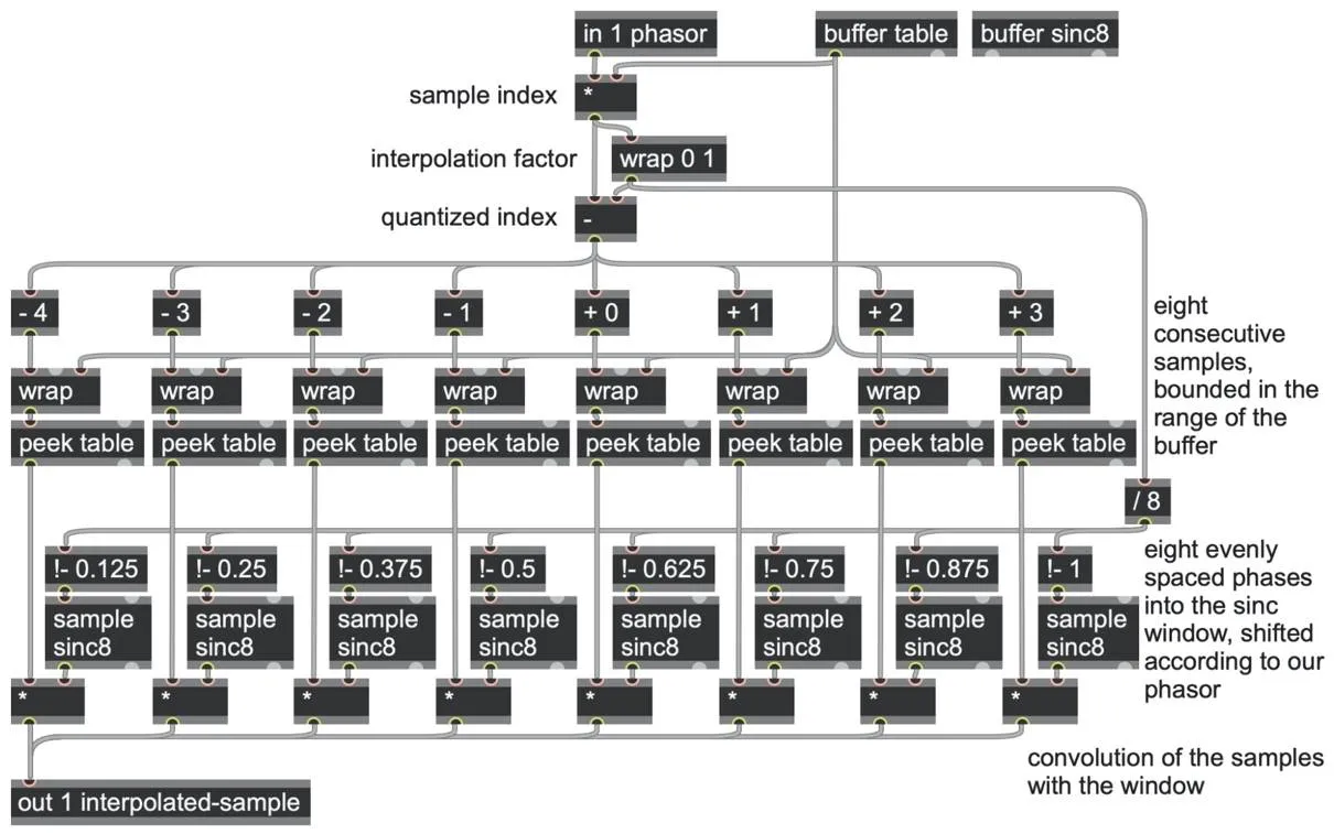
This is a dense patch, so let's walk through it step by step. First, our incoming phasor ramp is multiplied by the buffer length to get a sample index. We extract the fractional component of that using a wrap 0 1 operator, which will be used as our interpolation factor. We subtract this fractional part to get a quantized integer sample index, which is then routed to a series of subtractions and additions for the eight nearest integer sample indices, and we use a wrap operator on each one to ensure it is within the bounds of our buffer. These indices are then sent to the eight peek operators to extract our nearest eight samples in the wavetable.

Meanwhile, the fractional interpolation factor is divided into eight evenly spaced slices between 0.0 and 1.0, to select the appropriate corresponding points of the window, sampled using the sample sinc8 operators. Finally, each window point and wavetable sample is multiplied together, and the results are added up at the output to complete the convolution.

If the wavetable contains a saw shape and is played at around 450Hz, the spectrum will look something like the following:

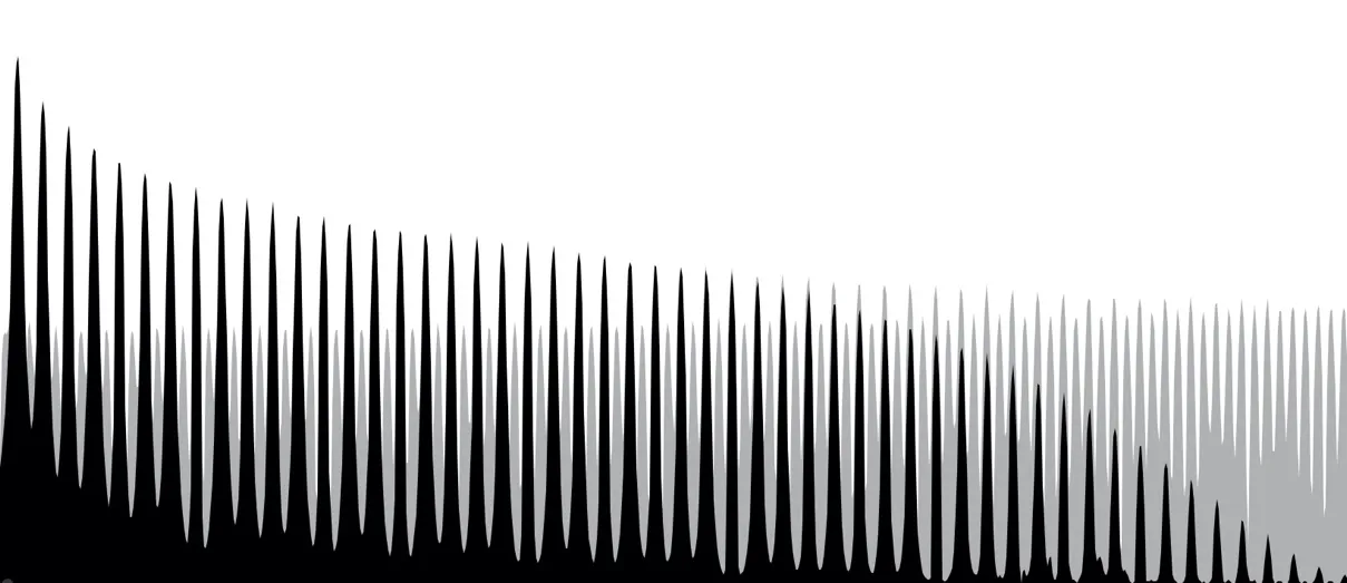
The black spectrum in the image above is the sinc interpolated waveform. The gray spectrum is the linear-interpolated waveform. Notice how the linear-interpolated waveform has a lot of extra energy between the saw harmonics: these are the aliased frequencies that sound particularly awful when the pitch is modulated, and they are present throughout the spectrum.[94] On the other hand, the sinc interpolated waveform has a clean series of harmonics that remain strong over most of the significantly audible range, then taper down to zero before they hit the Nyquist limit, preventing aliasing noise. The best part of this is that it doesn't matter at all what the wavetable actually contains. The same band-limiting will apply!

But there's a problem we still have to resolve, which becomes apparent as we change the driving phasor frequency: the spectral filtering moves with it.

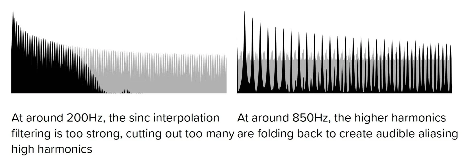
That's because our sinc filter is designed to work with a specific sampling rate; reading through the wavetable at a different phasor frequency means we are reading at a different sampling rate, and that would need a different sinc shape. It's expensive to compute these windowed sinc shapes continuously, so we're going to address this by extending our sinc interpolation with another technique called mipmapping.

Mipmapping

The technique of "mipmapping" is widely used in computer graphics to avoid the aliasing of high-resolution images rendered at low resolution output.[95] You've probably seen the result of aliasing in computer graphics in the form of Moiré patterns.

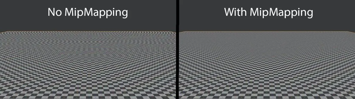
Look at the noise near the horizon in the image on the left (with no mipmapping) and compare this to the smoothness near the horizon in the image on the right (with mipmapping enabled).[96] In this graphic example, you see those noisy patterns because the detail in the checkerboard image far exceeds the sampling resolution of the pixels in the output image. Mipmapping helps solve this problem, and it can help us with our audio problems, too.

Here's how the graphics version of this technique works: a MipMap is a stack of versions of an original image, each of which is half the resolution of the version below. This forms a kind of pyramid, where each pixel of an image in one layer represents 2x2 pixels of the image in the layer below. Whenever we need to render the picture, we use whichever version has the closest resolution to what we want for the output, and we will know that it won't have too much detail to draw smoothly and thus won't get aliasing interference patterns.

We can use a similar approach to avoid aliasing in audio wavetable playback. Reading from a wavetable of a certain size at a certain frequency to render under a certain sampling rate is exactly analogous to reading from an image of a certain size at a certain distance under a certain rendering resolution. So, our MipMap can be a pyramid of wavetables, where each "higher" layer waveform has half the resolution of the one below.

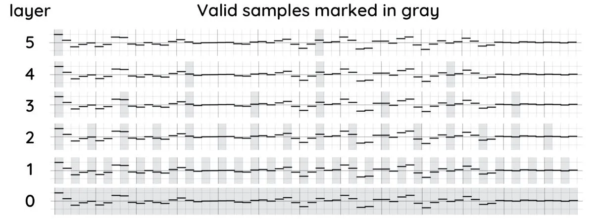
Starting from the bottom layer at full wavetable resolution, we could create the next layer above by simply "throwing away" every second sample (this is called "decimating"), giving us a waveform of half the resolution (half the total sample length). We can do that again and again for each layer going up the pyramid.

To keep our patch as simple and flexible as possible, we're going to compute the decimation on the fly during playback.[97] So, for the second layer, we want to read only every 2nd sample value (i.e., the even frames). For the next layer, we read only every 4th sample, i.e., only the data in samples 0, 4, 8, etc., and so on.

This sample spacing can be expressed as pow(2, layer), or more simply as exp2(layer). To apply this quantized spacing to our wavetable readers, we can use the same technique we have used for quantization elsewhere in this book: divide, convert to integer, then multiply again. That is, we divide our sample index by the spacing before we quantize it to an integer, and then multiply by the spacing again afterward (before each peek operator).

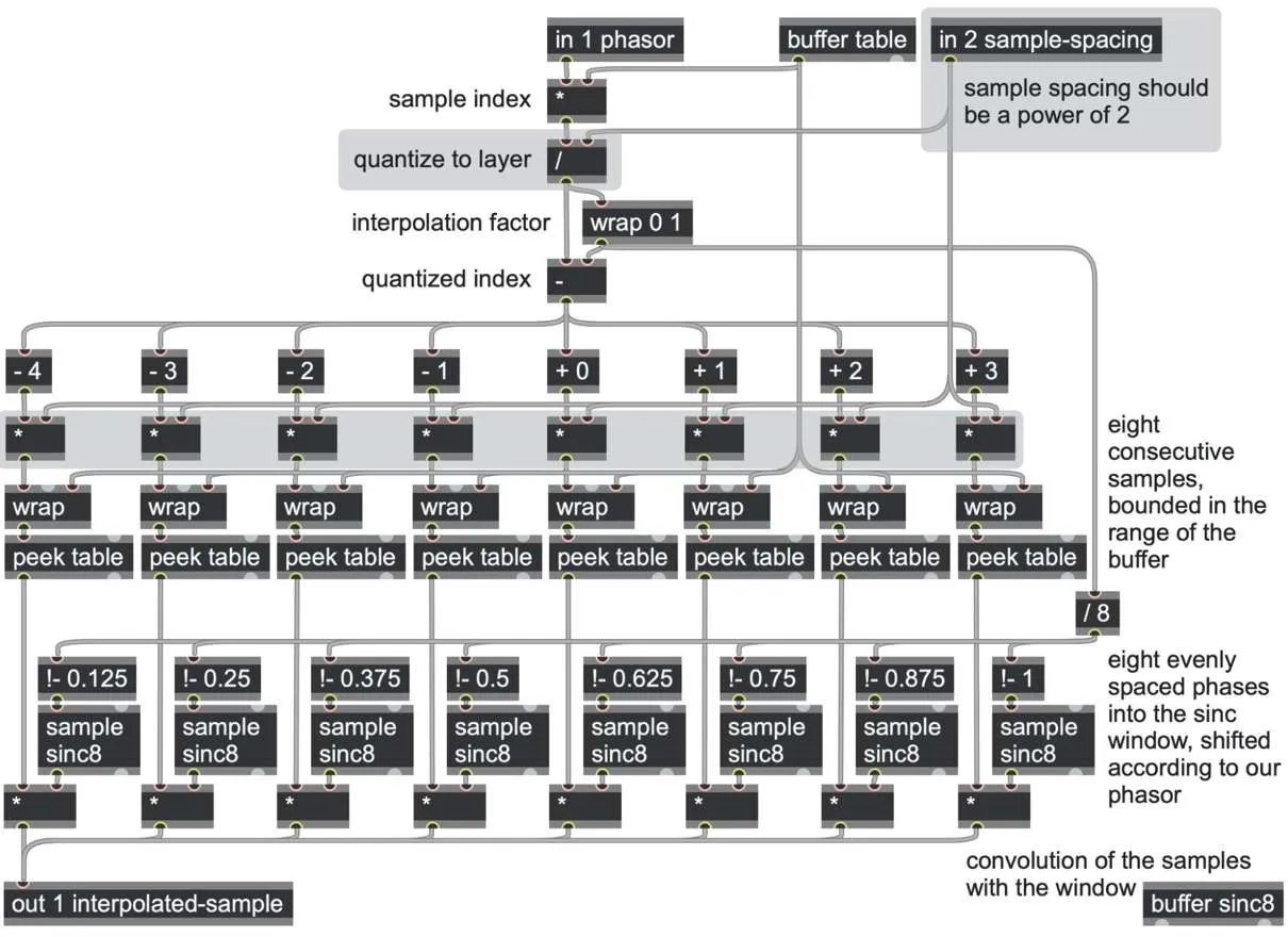
If you modify the in 2 sample-spacing control between 1, 2, 4, 8, etc. you will see the sinc filtering kick in at different octaves of the spectrum. So, all we need to do during playback is figure out which sample spacing (i.e., which waveform resolution) is appropriate for the playback frequency we are using to select the appropriate sample spacing to render at.

To do this, first we'll need to compute the relative sample density. This is just the rate of wavetable samples per sample in real time, so we can take our phasor's slope (using the go.ramp2slope abstraction) and multiply this by the wavetable resolution to get the density. We next want to quantize this to a power of two, which we can do with a sequence of log2, ceil, and exp2 operators. And that gives us the sample spacing we need.

The patch is getting quite large now, so we’ll put the sinc interpolation section into a gen @title sinc-interpolate subpatch.

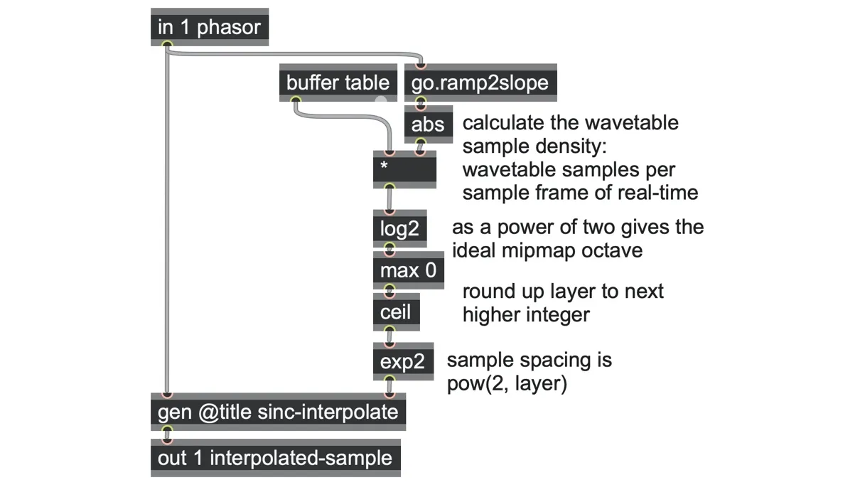
We also added an abs operator to ensure the patch works with phasors running backward and a max 0 operator because zero is the lowest possible layer we can render.

Now, no matter what frequency we play the wavetable at, the aliasing suppression remains in the higher regions of the spectrum! There's just one more refinement to make. If you wiggle the frequency around, add portamento or deep FM, you may notice a distinct change as the wavetable switches from one-octave layer to the next. It would be much better if we could crossfade smoothly between the two nearest layers according to which layer is nearer.

Once again, we can solve this by running two copies of our sinc interpolator and mixing according to the fractional step between layers.

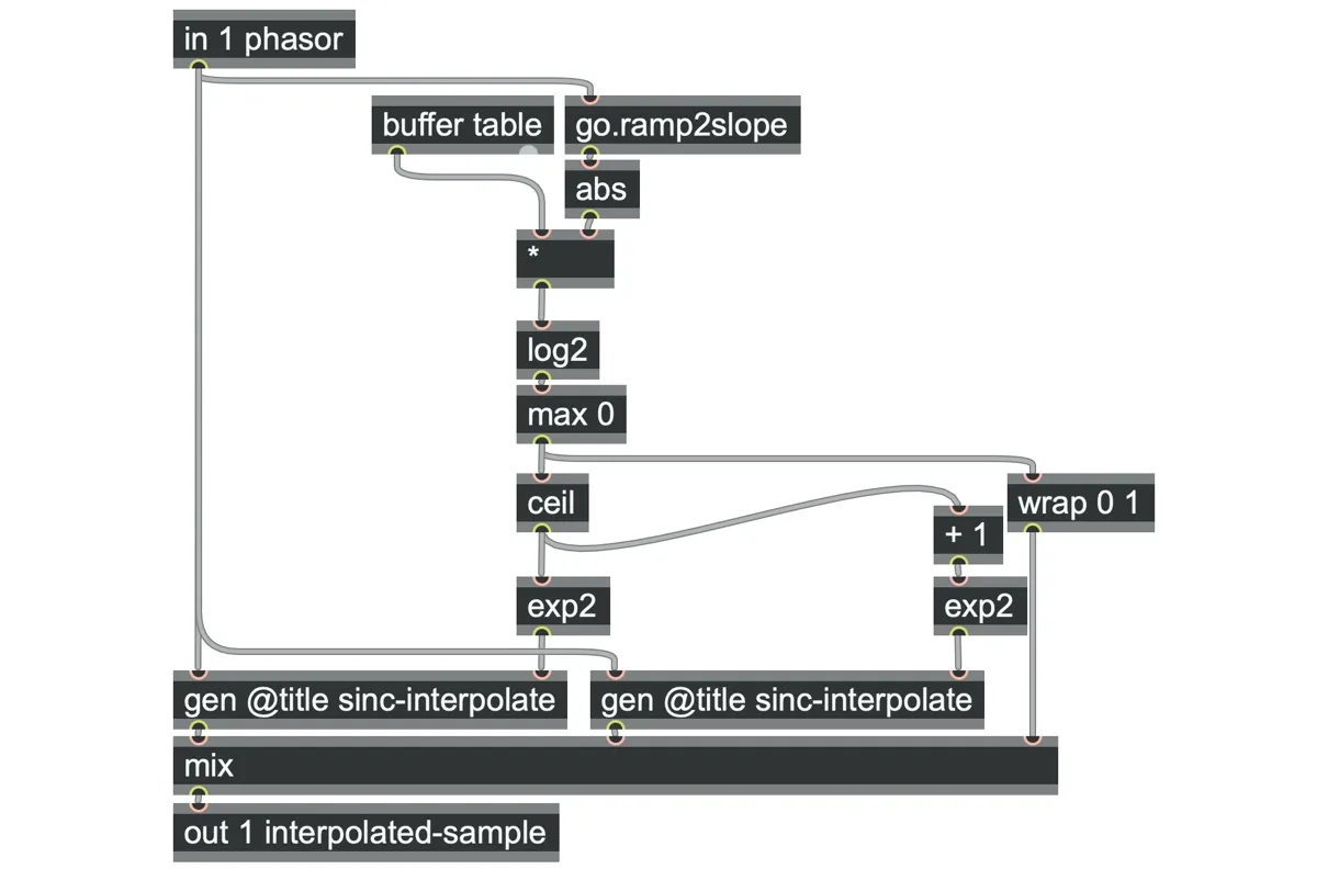
wavetable_sincmipmap_sample.maxpat

This patch can now be a drop-in replacement for a sample operator, and it will be bandlimited. What's more, this method remains bandlimited even under quite extreme audio rate frequency modulation, regardless of what data the wavetable actually contains!

With a little more patching, we can extend this to present the same interface as a wave operator. First of all, we'll need to add inlets to our sinc-interpolate subpatch to handle start and end sample indices, which feed into the wrap operators that constrain the peek operators.

We can then add inlets for the sample start and sample end positions in the main gen~ patch, and the difference between these will act as the effective resolution of the waveform.

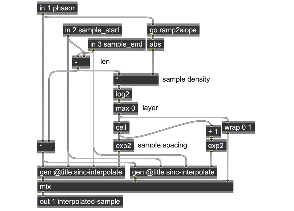
wavetable_sincmipmap_wave.maxpat

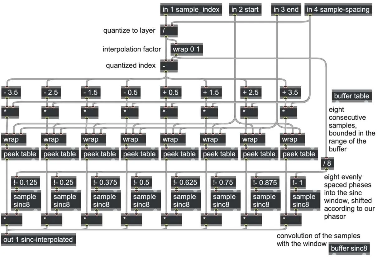
sinc-interpolate

Now, wherever we have used a wave operator before (including nearly all the wavetable patches in this chapter), we can replace it with our mipmapped, sinc interpolated subpatch above to get fully antialiased wavetable playback for any waveform, even while morphing between waveforms! Take a look at the mipmap_sinc_1D.maxpat and mipmap_sinc_2D.maxpat patches and explore applying deep modulation to them!

Wave terrains

As you modulate 1D, 2D, and 3D wavetables more deeply, you may observe that the output sound becomes more a function of the orbits through the space than of the content of the wavetable data itself. In this section, we're going to look at a closely related synthesis technique using 2D wave terrains, in which waveform data has almost entirely disappeared, and the orbits take center stage.

Wave terrain synthesis uses most of the same basic techniques as 2D wavetable synthesis, but in a slightly different way. Both include a dataset arranged over a 2D grid and an X and Y pair of signals to navigate this grid smoothly.

The primary differences are

• In a 2D wavetable, each point in the grid contains an entire single-cycle waveform. For a wave terrain, each point in the grid is just a single sample value.

• Typically, the number of grid sample points in a wave terrain is much larger than the number of waveforms in a 2D wavetable. For example, rather than a handful of single-cycle waveforms in each axis, a terrain may have hundreds or even thousands of data points on each axis.

The term "terrain" comes from the intuitive sense that the sample value at any grid point can represent a vertical height above the XY plane, which could be visualized like this:

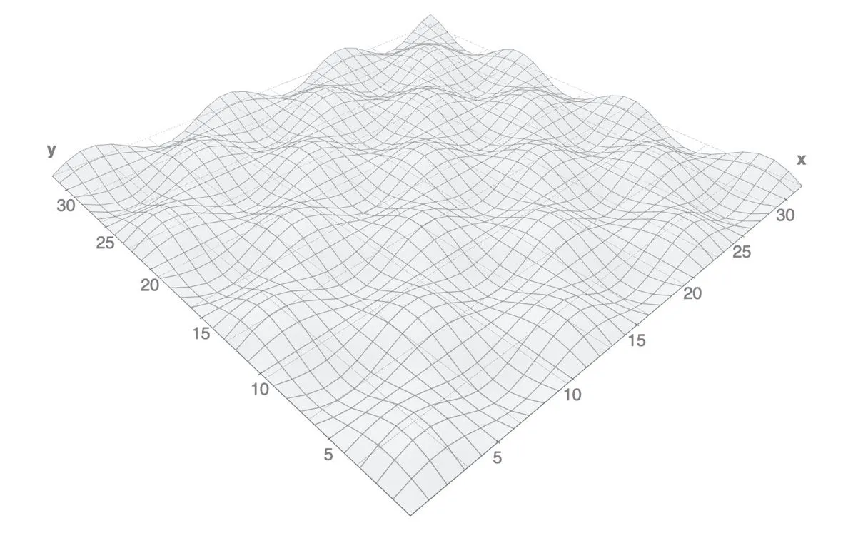
This particular terrain is a 32x32 grid of points, each of which has a height value computed as a function of sin(x*pi/5) + sin(y*pi/5), but any resolution and function of X and Y can be used.

The wave terrain algorithm uses two signal inputs X and Y to determine our location on this map, and the output signal is simply the height of the map at this location. The X and Y inputs normally modulate fairly smoothly to create a continuous traversal over the terrain. And, whereas for a 2D wavetable, you would normally expect neighboring waveforms to be similar, so that traversal over the space of waveforms (wavetable morphing) is mostly smooth, then for a wave terrain, you would normally expect neighboring sample points to be similar, so that traversal over the terrain is predominantly smooth.

In this way, wave terrain synthesis allows us to generate all kinds of interesting evolving and complex waveforms, whether as audio signals or as lower-frequency control signals. In this section, we're going to look at a few different ways to generate interesting 2D terrains and explore some different ways to traverse these surfaces.

But first, we'll start with a basic terrain reader patch, which looks like this:

gen @title terrain-reader

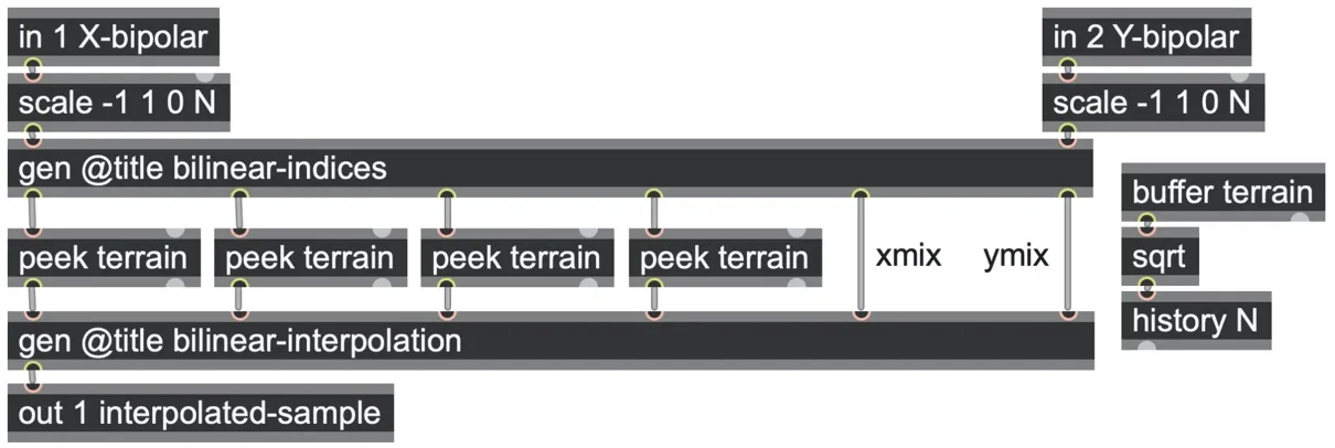
As with multi-dimensional wavetables, our wave terrains will be stored in a regular one-dimensional buffer operator. We'll assume that our terrains are square, with the same number of samples across each axis, so we can calculate our resolution as the square root of the buffer length using the sqrt operator and store it in a history N operator so that the variable "N" is available for use throughout the patch.

To read from this terrain, we'll need a way to convert an X and Y coordinate into an index into the buffer, so we can read the data it contains. For wave terrains, it can be handy to work with bipolar signals for X and Y, so the first thing we do is convert these to axis coordinates using scale -1 1 0 N operators.

To interpolate between samples on the terrain smoothly, we can use the same basic approach as we did for the morphing 2D wavetables example: finding the four nearest indices, computing outputs at these indices, then crossfading the results. In fact, we can use exactly the same bilinear-indices and bilinear-interpolation subpatches as we used for the morphing 2D wavetables. Since the terrain contains only a single sample value at each of these points, we can directly feed the indices into four peek operators to retrieve the nearest terrain values and send those on to the bilinear interpolation. (We're using non-interpolating peek operators here because we'll be performing our own interpolation in the bilinear-interpolation subpatch.)

Now that we have a reader, we'll need to generate an X and Y pair of signals for its inputs. One of the simplest traversals we can try is a basic circular path (or "orbit"). Circular paths are popular for wave terrain traversal because they produce periodic results by definition.

The poltocar operator provides us with a simple way to generate a basic circular traversal. The name means polar to Cartesian coordinates, which simply means that it converts a radius and angle input into an X and Y output.

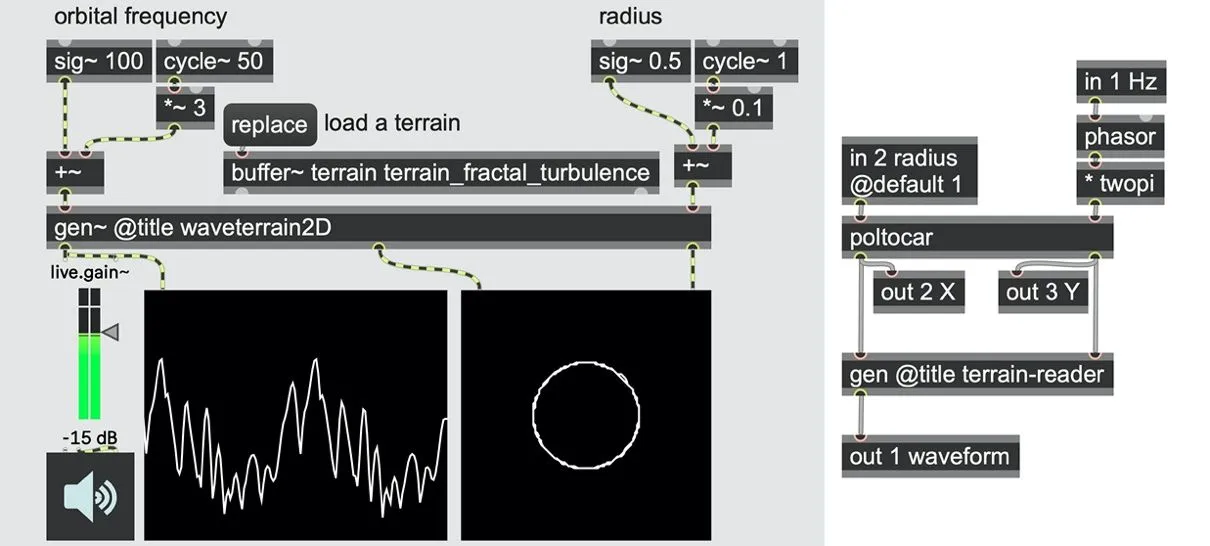
waveterrain_2D.maxpat

We specify the radius of the circle we want to create, as well as an angle in radians (ranging from 0.0 to 2π). In the patch above, we put this into continuous rotation by driving the angle input with a phasor scaled up to 2π radians using a * twopi operator.

Finally, we need some terrain data to load into the buffer~ terrain object. In the next section, we'll describe some ways to generate terrain data procedurally; but to get a quick start, we've provided a folder of audio files located in the media folder of the software that accompanies this book, generated at a 1024x1024 resolution.

It's worth exploring the orbital parameters to get a sense of how it changes the output waveform. The angular rotation of the phasor is what provides the fundamental frequency for the waveform at the output. There is often also correspondence between the radius and the brightness of the output sound—this is because, with a smaller radius, we are effectively moving over fewer distinct samples in the terrain—which is like reading from a wavetable with a lower resolution and thus less space for higher harmonics.[98]

Generating terrains

If you want to generate your own terrain, all you need is to create a function that computes the terrain's height value ("Z") from the 2D grid coordinate in X and Y. Then, with a bit of patching (and codeboxing), we can fill a buffer~ with samples of this terrain function and save it to a wave file.

To start, we will want a buffer~ terrain object in the parent patch that uses the @samps attribute to set the number of samples in the buffer. The buffer length in samples should be a square of the dimensions of the terrain we want to generate. Generally speaking, a larger buffer size will generate a more detailed terrain whose output can have more high-frequency response when "read." For example, for a 512x512 terrain, we would use buffer~ terrain @samps 262144, and for a 1024x1024 terrain, we would use buffer~ terrain @samps 1048576.

As before, we can refer to this buffer~ in gen~ using a buffer terrain operator and derive our axis resolution from the square root of its length using the sqrt operator, which we store in a history N operator.

We’ll also add a codebox to do our computations to fill the terrain, which looks like this:

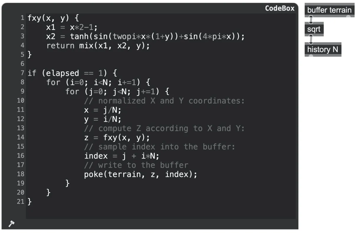
Let's step through that code. First, we have the function fxy(x,y)that defines our terrain. You can put whatever mathematical calculations you want into here; all it needs to do is return a height value between -1.0 and +1.0 according to the current X and Y position. That said, you probably want to find a terrain that strikes an interesting balance of complexity—not so simple that it becomes boring, but also not too random that it becomes noise—the changes between one grid point and the next should be relatively small for the most part to create an undulating terrain. In the codebox above we just made up something that seemed interesting to us: a mix across the Y axis between a sawtooth wave (x1) and a tanh-waveshaped sum of two sines across the axes (x2).

Defining the function doesn't do anything yet—not until we actually invoke this function in the main body of the code. The main body starts with if (elapsed == 1), which is just a simple way to ensure that all the code inside the next block (i.e. between the next "{" and the matching "}" brackets) only runs once. (The elapsed variable (and operator) always outputs the number of sample frames that have passed since the patch loaded, which will only equal one once.) If we didn't do this, the patch would be trying to regenerate the waveterrain on every passing sample frame, which is computationally expensive and unnecessary.

Inside this if block, we have two nested for loops: one stepping N times for each row in the Y axis, the other stepping N times for each column in the X axis, making the innermost body of code run NxN times altogether. Each pass through the innermost loop will calculate a different Z value for each XY point in the terrain and store it at the correct location in the buffer. The code first computes normalized X and Y coordinates (running from 0.0 to 1.0) by dividing both step counts by N. We'll use those normalized coordinates in the fx(x, y) function call to compute the height z for this particular grid cell. Next, we compute what the sample index will be into the buffer for this grid cell (i.e., where to write the value z to), which is the same calculation we used before for the 2D wavetable: index = j + i*N. And finally, we plug in the index and z value into a poke operation to write it to the buffer terrain.

Remember, you can use any function that refers to the X and Y values to derive the single Z value—feel free to experiment with functions of your own! If you find a terrain you like, send a "writewave" message to the buffer~ object in the parent patch to save the data as a WAV file.

Basis Function Generator (BFG) terrains

As an alternative, we can also generate terrains by using the extensive matrix generation capabilities of Jitter. For example, the Jitter object jit.bfg can generate matrix data for a wide variety of interesting mathematical surfaces (BFG here stands for basis function generator). Working with Jitter is not the focus of this book, but this is such a useful source of terrains that we included an example patch to demonstrate generating landscapes for wave terrain synthesis.

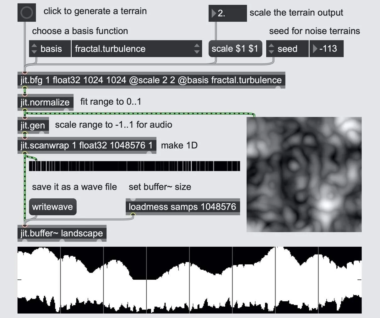
waveterrain_generate_BFG.maxpat

The jit.bfg object is configured to set the plane count (1), the matrix type (32-bit floating-point values), and the dimensions of the terrain (1024x1024). In addition, we set a default scaling value (@scale 2 2) and the basis function (@basis fractal.turbulence), which we can override with attribute menus.

When the button is clicked, the jit.bfg outputs a matrix, which we will process and convert to store in a wave file. First, we normalize the results to get an optimal spread of output values between zero and one and then use a jit.gen applying a scale 0 1 -1 1 operator to scale the matrix contents to the -1.0 to +1.0 range we expect for audio. This outputs a 2D 1024 X 1024 single-plane matrix of audio-range values, which we convert to a 1D matrix of length 1048576 via the jit.scanwrap object, to be stored in a jit.buffer~ object.

The useful thing about the jit.buffer~ object is that we can treat it exactly like any buffer~ object (we can even reference it by name for the gen~ object's internal buffer operator, for example). This means we can send it the writewave message, which will let us save its contents to a .WAV file on disk.

Navigating data space

For the last section of this chapter, let's look at some more interesting ways of moving around a 2D data space by generating related X and Y signal pairs. We'll give these examples in terms of wave terrain synthesis applications, but bear in mind these same orbit generators can also be used for the X and Y parameters of a 2D wavetable patch or, indeed, any other algorithm that works with two related inputs.

Our first wave terrain patch used a circular orbit derived from a poltocar operator. While such circular orbits work fine for an initial example, there are many ways of making that circular traversal much more interesting. For example, we can nudge the orbit away from the center simply by adding more signals to the signal outputs of the poltocar operator.

We can extend this to a kind of parallel modulation approach and create a "double orbit" simply by adding two poltocar operations together. Setting the frequencies and radii to different values can produce interesting results, including paths like a moon orbiting a planet orbiting the sun, as well as much more extreme excursions!

However, when adding two orbits together, it's quite possible that the signals can go outside the -1.0 to 1.0 range that a wave terrain reader expects. To avoid this, we have a few options.

• We could send the results through fold -1 1 operators so that the signals will mirror at the edges.

• We could send the results through wrap -1 1 operators to have it jump around to the opposite edges or clip -1 1 for hard clipping at the boundaries.

• We could apply any of the sigmoid waveshapers from Chapter 3 to compress the waves as they get nearer to the edges.

We could even use param and selector operators to vary the method we use.

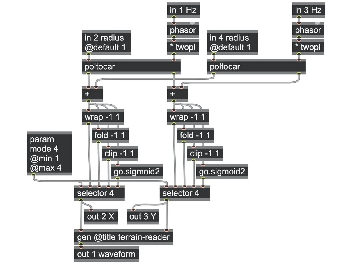
waveterrain_2D_doubleorbit.maxpat

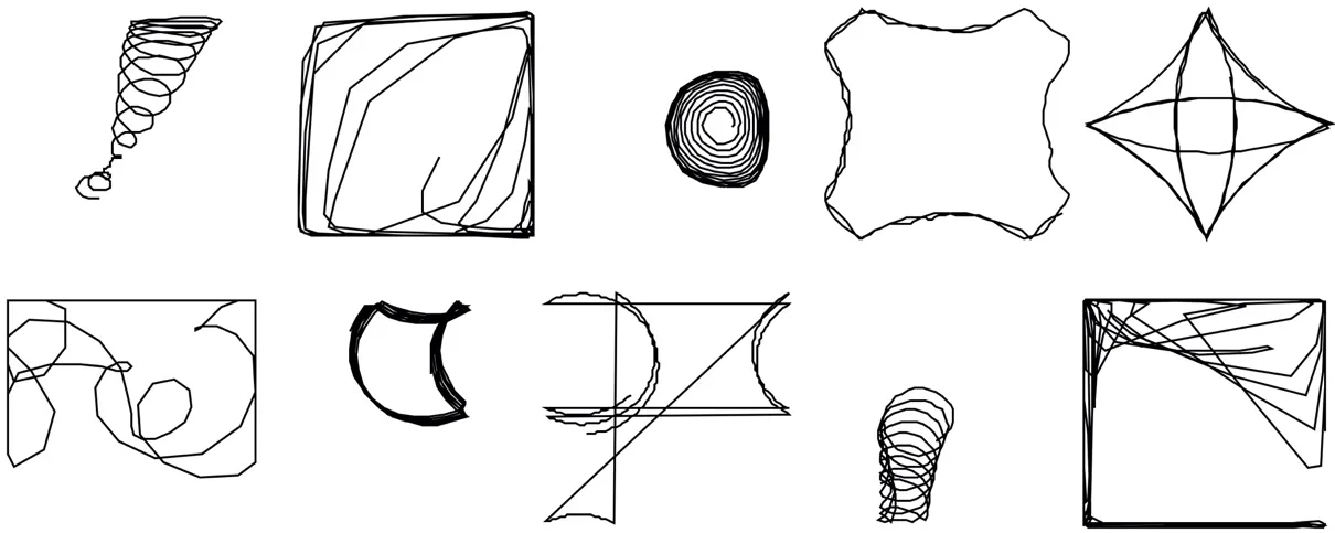
Here are a selection of eccentric traversals this can produce.

Circular orbits aren't the only choice. Any mostly smooth sequence of X & Y values in the range of -1.0 to +1.0 can yield workable results. For example, we can use simple accumulators into fold operators to produce a variety of triangle-like waveforms independently for X and Y.

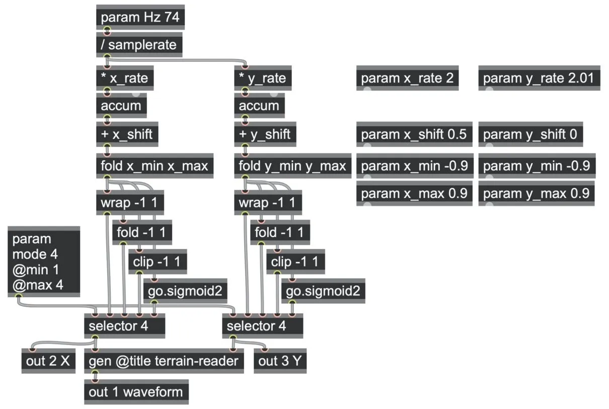
waveterrain_2D_carom.maxpat

As long as the X and Y rate parameters are similar, this patch will produce 45-degree angle traversals that appear to "bounce" off the min/max boundaries; but once the rates diverge, the angles change, and the diagonal shape breaks into weaving motions. Any modifications of the boundaries produce more complex patterns and will also "retune" the output. The caroming traversal can produce all kinds of results.

You might wish to experiment with having multiple versions of this patch traversing different areas of the same wave terrain at different rates.

Polygonal orbits

We've seen circular as well as diagonal orbits; what about traversals that describe regular polygons like triangles, squares, and pentagons? In fact, we can do this using a phasor-driven poltocar operator as before. The difference lies in the way we derive the radius input. If we can modulate the radius with just the right function, we can effectively inscribe the polygon within the circle—and it will inherit the periodicity of that circular basis too.[99] That is, we want a function that gives us the radius we need from the angle we have. You could think of this as a kind of precisely-tuned amplitude modulation or waveshaping of the radius.

The waveshaping will repeat N times around a circle for an N-sided polygon. For example, a triangle has three sides, so we need to shape the radius with the same curvature three times as we go around. To patch this up, we'll add a second phasor running at N times the angular frequency (which, therefore, also adds an audible harmonic). You can thus think of this param N as a modulator to carrier ratio.

We then apply some scaling math that lets us use this as the amplitude of the oscillator, which we send to the radius (left) inlet of the poltocar operator.

The equation of a unit polygon of N sides (and N vertices) in polar coordinates is the ratio of the angle between vertices (which is cos(pi/N)) and the current angle, which runs from -pi to +pi over each vertex:

r = cos(pi/N) / cos(angle/N)

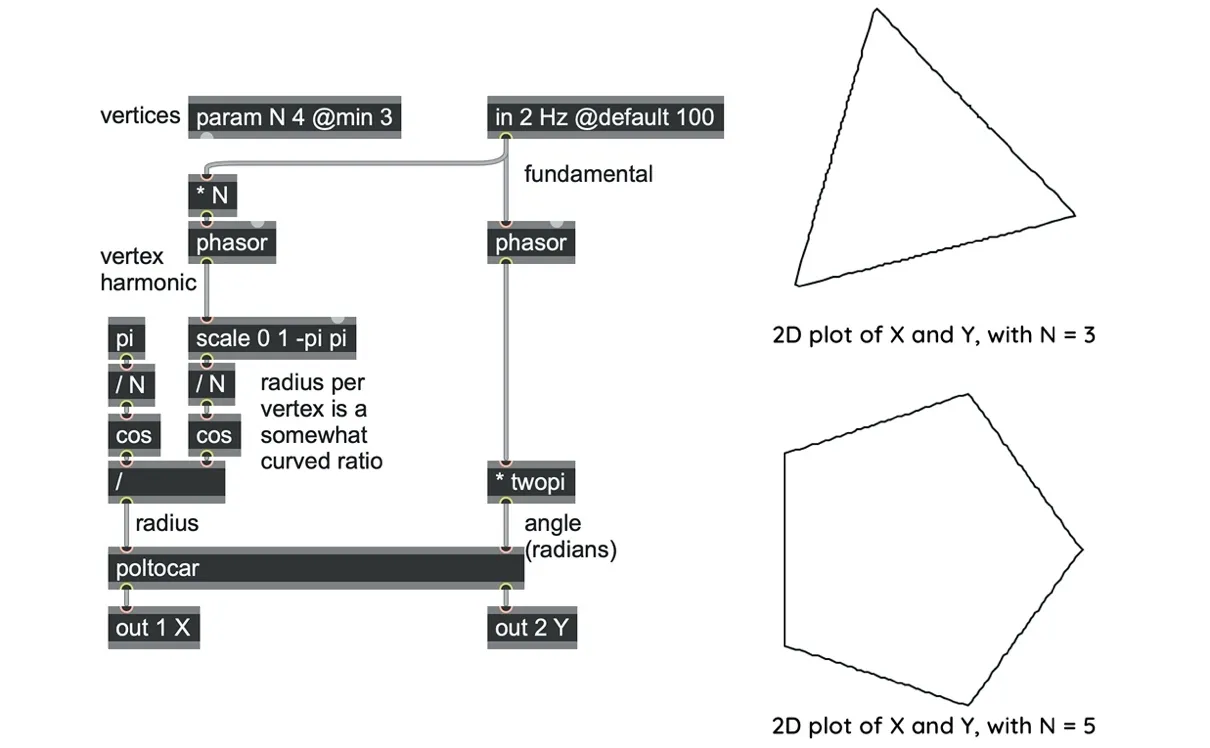
A basic polygonal oscillator patch

This can be extended in a few ways. There's no need to limit N to whole numbers. For example, if we set N=3.01, we will get a triangle shape that appears to spin in space, as each time around, it overshoots slightly. This is not unlike the benefit of slightly detuned oscillators and modulators we saw in Chapter 8. Suppose we don't want it to spin but instead want "partial" polygons. In that case, we can do the equivalent of oscillator sync and reset the vertex phasor to zero whenever the fundamental phasor resets.

We can also add a separate phase modulation offset "P" to the fundamental phasor output, which will effectively give us direct control over the rotation of the shape in space.

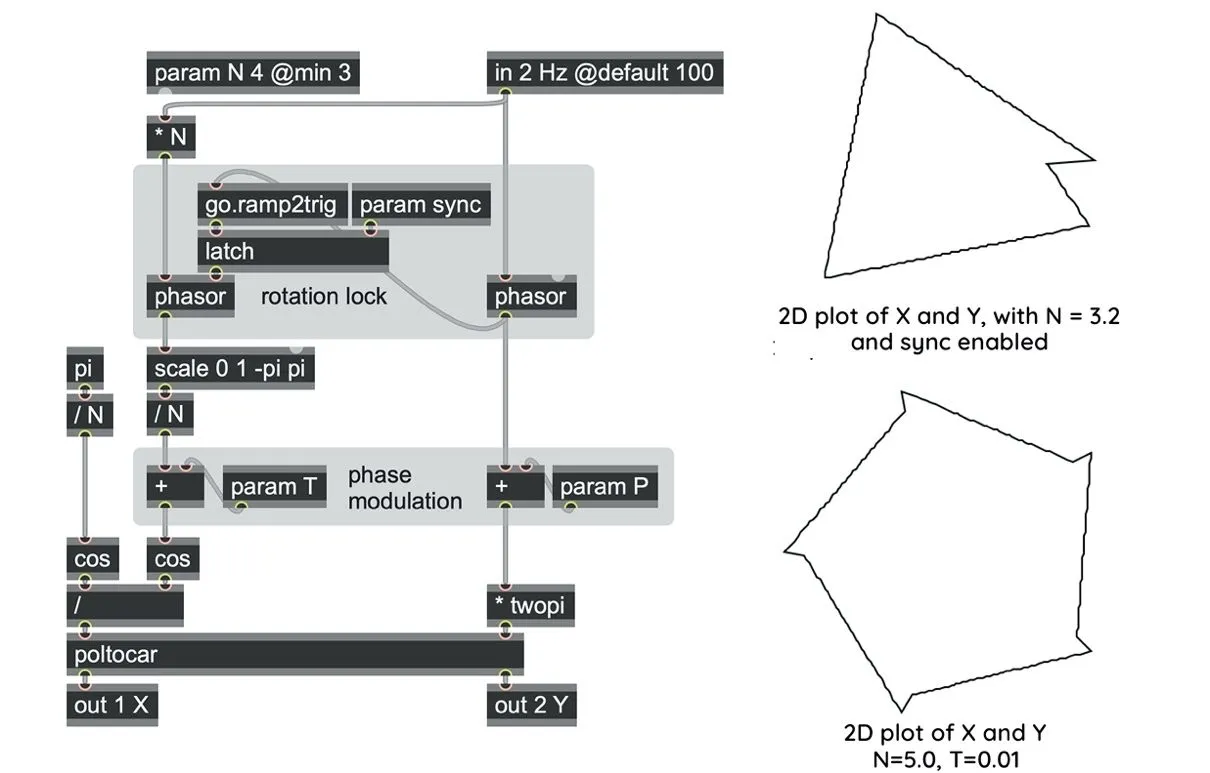
Polygonal synthesis with sync and phase modulation

Adding a phase modulation offset to the per-vertex phasor (param T in the patch above) does something different. It "kinks" the straight side out, disrupting the output function in a way that repeats itself for each "section" of the polygon. It looks a bit like adding "teeth" to the shape.

Turning up this param T can easily make the shape expand beyond the -1.0 to +1.0 signal range, so once again we might want to add some kind of signal limiting here. And once we have limiting, it makes sense to add a param drive to push it.

For example, in the patch below we feed the potentially overdriven radius through a fold operator whose outer bound is 1.0 but whose inner bound is dependent on the angle, to keep the folding signal closer to the original shape's bounds.

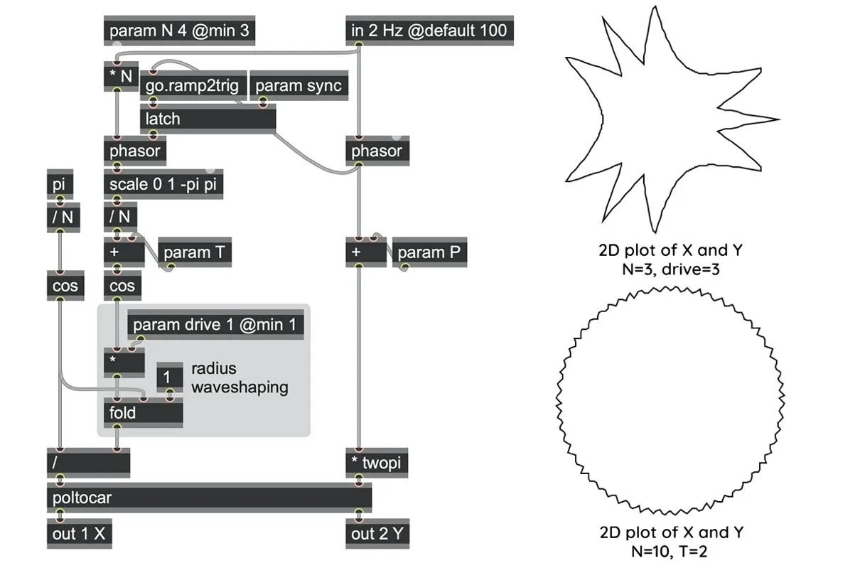
Polygonal synthesis with wavefolding, in polygonal.maxpat

There are lots of other things you could try in this kind of patch—perhaps sigmoid waveshaping to bow out the straight edges; perhaps bitcrushing/quantizing to step the radius; perhaps amplitude modulations, filtering, or any other signal processes! You can also try converting some of the param operators to regular in operators to feed with audio-rate modulations. Don't be afraid to experiment!

Although we've introduced these orbit generator patches for traversing 2D wave terrains or 2D wavetables[100], they are also very useful as modulation signals for other kinds of processes, such as frequency modulation and phase modulation patches, as well as for generating audio signals in their own right of course!

Taking things further

In this chapter, we've looked at many ways to generate more interesting waveforms by navigating data sources, and there are many ways you can take these ideas further.

So far, we have been using monophonic wavetables and terrains, but a buffer (or data) operator can be multi-channel, and so can the readers. For example, any of the sample, wave, or peek operators our patches used can be made stereo by adding an @channels 2 attribute, or more simply adding the argument "2" after the buffer name, such as wave tables 2 or peek terrain 2. Then, any patching downstream of these (such as the bilinear-interpolation subpatch) just needs doubling up to process each channel's output. We can also get interesting stereo output from a monophonic wavetable or terrain by running two copies of our patch side by side, feeding them related but slightly different indexing signals. For example, we run two terrain-reader patches and send the second terrain-reader the same X but an inverted Y (i.e., multiplied by -1.0).

As a wavetable's (or wave terrain's) data becomes more complex, it adds more higher-harmonic energy to a signal, sometimes at the cost of losing some of the fundamental frequency energy—this can be problematic for use as a bass, for example. A straightforward solution here is to add a simple waveform (sine, pulse, or saw) in parallel, driven by the same phasor that is driving the wavetable. (Or for wave terrains, using the same phasor that drives the angular rotation).

From the point of view of these core phasor operators, both wavetables and wave terrains become simply interesting functions of phase, just as was the case for the various frequency and phase modulation patches in Chapter 8. So, naturally, you can explore modifying those FM and PM patches, replacing the * twopi and sin operators with wavetable oscillators. There's an enormous amount of sonic complexity available here, and if you're using the sinc interpolated, mipmapped wavetables, they will handle pretty extreme modulation without aliasing. Similarly, you could explore some of the FM and PM structures for the polar (poltocar-based) oscillators. Simply adding frequency modulation to the radius and angle inputs can pick out some mesmerizing orbits.

Perhaps you might think about how to extend orbit generators to 3D to drive a 3D wavetable oscillator. Or, if you're feeling ambitious, think about how to generate and navigate 3D voxel terrain.