Chapter 1:
Patching One Sample at a Time

This book is all about the astonishing things you can do—and the insights you can find—when you work at the atomic sample-by-sample structure of digital audio.

The immense possibilities of digital signal processing (DSP) are often inaccessibly black-boxed in music software, and sometimes also shrouded in a mystique of complexity. In this book we’ll use gen~, which lets us work directly at the sample level through visual patching (or by coding if you prefer to) and hear the results immediately at every edit. Our aim is to crack open these black boxes, revealing how working at the sample level is not only easier to reason about, but also far more open to experimentation.

Whether you are a musician, sound designer, composer or some other sonic experimentalist, we hope that demystifying a wide selection of musical signal processing techniques, and showing how they are put together from a few common structures, will make it easier for you to imagine and explore variations, hybrids and completely new directions of your own. This book is therefore also about developing useful things to think with: design patterns, techniques and subcircuits to help you approach sonic signal processing at the sample level and bring amazing new things to life. Starting from the simplest beginnings, we’ll develop

• algorithmic rhythm generators, beat slicers, Euclidean sequencers

• morphing LFOs, wave shapers, bit-crushers and gliding quantizers

• chaotic systems, stepped and smoothed noise and chance operations

• a wide palette of filters and delay effects

• a plethora of phase and frequency modulation algorithms

• formant, pulsar and polyphonic granular synthesizers of various kinds

• bandlimited virtual analog and wavetable oscillators capable of intensive modulation

…and more in the extensive software package provided with the book.

Before we dive into exploring these topics and projects, we think it is helpful to share a couple of insights into the nature of digital signal processing of sound. In all digital audio systems, time passes in discrete steps. Throughout this book, we’ll refer to those discrete steps as sample frames. These sample frames divide and represent time in terms of the audio sample rate — typically 44,100 or 48,000 sample frames per second of real time, which is fast enough to represent pretty much any sound humans can hear. Every digital audio signal is therefore just a stream of numbers.

Within a typical audio plugin for example, these audio streams pass in a flurry through sequences of a few math, logic and memory operations, to produce transformed signals at the output. To make signal processing efficient, these operations will have been pre-compiled from a language like C++ into native code. However, this also makes them less flexible: it’s not possible to change the operations inside and hear the results right away (and you would also need to learn a language like C++). Moreover, they are processed in batches of time, sometimes called “buffers” or “blocks” or “signal vectors” of sample frames. This means you can’t join them up in feedback circuits shorter than this signal vector size. As we’ll see in this book, feedback circuits are fundamental to most audio algorithms, and building feedback circuits as short as a single sample frame is essential to many filters, oscillators, physical models, chaotic processes, and more. The gen~ patching environment was designed to resolve these problems.

What is gen~?

At first glance, gen~ is just another object that can be added to a Max or RNBO patch, where it can send and receive audio from other objects you connect it to. What makes a gen~ object different is that you can open it up to view its internal circuits and edit what they do, right down to the lowest details of sound signal processing at each passing sample frame. As such, gen~ is also a distinct patching environment (and language) devoted to audio processing and musical programming at the sample frame level.

At the same time, the gen~ environment retains the benefits of flexible patching and native efficiency. With every edit as you work, behind the scenes it is immediately generating and compiling efficient native CPU code for the whole patch. That means can you hear and interact with new sample-level programs and algorithms as you develop them on the fly. It also means that gen~ lets you work at this level without needing to use a complex language like C++, but it can still give you the high performance of compiled C++ code.

What’s more, and what this book is really about, it means we can think about and develop sonic signal processes at the very level of sample-by-sample operations they are made of. Working at this level means we can define processes—including feedback down to a single sample frame—that are either very difficult or simply impossible any other way. We also think that it makes reasoning about and exploring sonic signal processing much easier. Starting from a humble set of operators you can build up a very flexible library of useful subcircuit “abstractions” that you can combine into powerful yet efficient patches. We’ll be doing this throughout the book.

(And, although this isn’t the focus of this book, it’s worth mentioning that if you make patches that you like, you can also take these algorithms with you. The entire contents of a gen~ object in a Max or RNBO patch can be embedded in a Max for Live Device, or it can also be exported as C++ code for use elsewhere. A RNBO patch that has gen~ objects inside it can also be exported into targets such as audio plugins and embedded hardware devices, or as web-native or C++ code.)

Using this book (and the software that comes with it)

This is a book full of many different circuits and projects, as well as insights and habits of thought. We don’t assume that all readers will read from start to finish, so we’ve tried to structure chapters and sections in ways that will help you to find areas that are of specific interest to you. At the same time, we have provided links and cross-references throughout the book to connect between foundations and possibilities and reinforce the ideas and techniques from the part you’re currently reading.

We designed this book to serve equally well whether as a companion for self-study or as a resource for educational situations. We have written it so that you don’t need much knowledge of math at all, and we don’t expect you to be a coder or even an experienced gen~ user, but the book does assume that you have a little experience of patching with Max or RNBO and know how to create and edit a gen~ patcher. If you’ve never used gen~ before or you’re feeling uncertain, the “gen~ for Beginners” tutorial series on the Cycling ’74 website (https://cycling74.com/tutorials/gen-video-tutorial-series) will provide you with all you need.

The book also comes with a Max Package including all the patches we build in this book, and more. You can download it from:

cycling74.com/books/go/resources

All you need to do is unzip the downloaded file and place the result in your Max Packages folder (e.g., “Documents/Max 8/Packages” or “My Documents/Max 8/Packages”).

A Bestiary of signals and operators

Before we dive into exploring projects and patches, we think it is helpful to recall the nature of sonic signal processing as a combination of signal streams and operations, which within a gen~ patch all happens one sample at a time.

The result of this has three results.

• Every patch cord is a signal that is updated with every sample frame of passing time.[1]

• Similarly, every operator also updates at this same sample rate, one sample frame at a time.

• Moreover, the entire patch also moves forward one sample frame at a time. This is what lets us perform essential “single-sample” feedback processing, which we do all the time.

For the remainder of this chapter, we would like to introduce the most common kinds of signals and operators we use as building blocks to generate and organize ephemeral digital sound. You can think of it as a bestiary or cast of likely characters if you like. We hope that this will help you to better understand just about everything else in the rest of this book.

Signals

Patch cords can carry audible signals, but they don’t have to: signals can carry any numeric values, and their behavior and purposes can be quite varied. So, when you think about a signal, it’s often helpful to consider its main characteristics.

• Rates of change

  • Does the signal change at audible rates, more slowly, or not at all?

  • Are those changes periodic, sporadic, complex, or stochastic (random) over time?

• Shapes (and slopes) of change

  • Does the signal move in stepped, sloped, or curved segments, or does it have a more complex shape? How steep are the slopes, and how tight are the curves?

• Ranges of values

  • What are the lower and upper limits of the signal (if any)?[2] Is the range composed of only positive values (unipolar), or does the range include negative values (bipolar)?

  • Can the signal take any numeric value in this range, or is it limited to whole numbers only (“integers”), to a handful of specific values, or only 0.0 or 1.0 (“logic signals”)?

• Kinds of value

  • Does the value represent a linear or cyclical idea? Values such as clock-face time and angles, as well as the phase of an oscillator or a metric rhythm, are all cyclical—when you pass the upper limit, you wrap back to the lower limit (e.g., an angle of 365° is the same as an angle of 5°).

  • Do the values correspond to specific units such as time (milliseconds), frequency (Hz), loudness (decibels), MIDI note numbers, etc.?[3]

Let’s take a closer look at some of the most common variants of the signals we work with in terms of their rates, shapes of change, ranges, and kinds of value.

Audio signals

An audio signal is one that we can potentially hear. This means that the signal oscillates up and down hundreds or thousands of times per second.

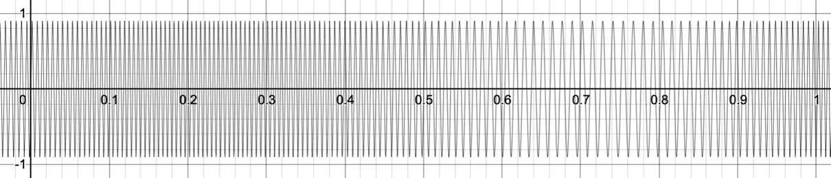
This graph shows a sine wave oscillating up and down at 100-200Hz (100 to 200 oscillations per second), which could be created using a cycle operator. (The term "Hz" is short for Hertz, which is a standard representation of frequency. So, 100Hz simply means 100 oscillations per second.)

All audible signals are in motion, jumping up and down one way or another. It is primarily the repetitive periodicity of their movement that imparts pitch and their distribution of shapes that colors how they sound (their timbre).

Normally, audio signals move in a bipolar way (which means, they can swing both negative and positive), ranging from -1.0 to +1.0 at their loudest or over a narrower range for quieter sounds. If audio signals go below -1.0 or above 1.0, they may be clipped or distorted by your audio hardware.

The fastest audio signal a digital system can represent is one half of the sampling rate (since it takes two samples per period to make an oscillation!)—this is called the Nyquist limit. At a frequency of 48,000Hz, the Nyquist limit of samplerate/2 is 24,000Hz, which is higher than humans can hear.

Low frequency oscillations (LFO)

If we slow oscillations down well below around 30Hz, we will no longer hear them directly, but these kinds of signals can be extremely useful for animating parameters of operations–common musical examples include vibrato and tremolo. LFOs are also often bipolar but do not need to be, nor do they need to stay within -1.0 to 1.0 limits.

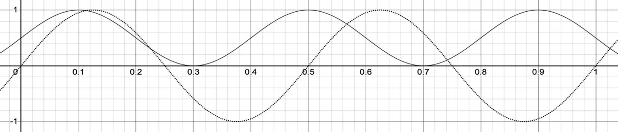
The dotted line in the previous illustration shows a bipolar sine wave oscillation at 2Hz (two cycles per second), which could be created using a cycle 2 operator. The solid line is a unipolar sine wave (sweeping between 0.0 and +1.0) at 2.5Hz.

Unipolar ramp (phasor)

A special unipolar function is the ramp from 0.0 up to +1.0 (or in reverse, from +1.0 down to 0.0). These kinds of ramps can be thought of as a universal primitive of repeating change and are used in almost every section of this book, but especially in Chapter 2.

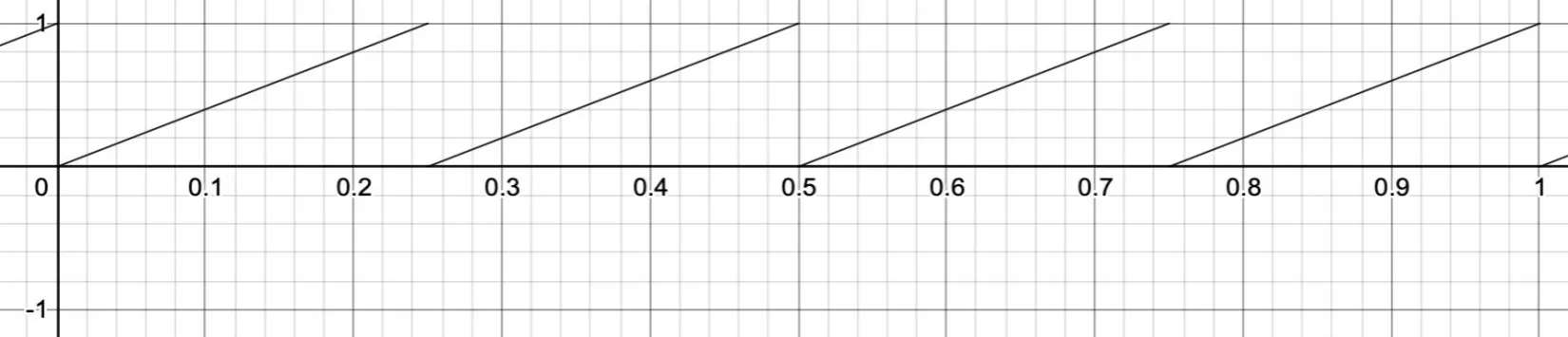
This following graph shows a ramp repeating at 4Hz, as produced by a phasor 4 operator.

Unipolar envelopes (and windows)

The unipolar range is very useful as a multiplier for any other signal, since multiplying with the upper limit of +1.0 will preserve the signal; multiplying with the lower limit of 0.0 will silence it; and anywhere in between will attenuate the signal (make it quieter). Accordingly, a smooth ramp up to +1.0 and then back down to zero is often used to “envelope” or “window” the dynamics of a sound event, smoothly shaping and containing its activity.

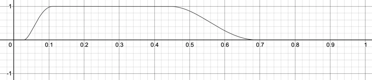
Just like this graph, natural envelopes usually rise faster and fall more slowly, but not always. We’ll look at ways to create envelopes and windows in Chapters 3, 4, and 11.

Stepped signals

By “stepped signals,” we mean a signal that flatly holds a steady value for a while and only occasionally changes to a new value. (Remember, operators and signals always run at the sample rate, so even a stepped signal is still a continually running stream of samples—it’s just that within one step all the sample frames have the same value.)

In this graph, the solid line is a signal that holds a value of 0.4 for a while, then jumps to 0.8 for the remainder, while the dashed line holds a value of zero throughout.

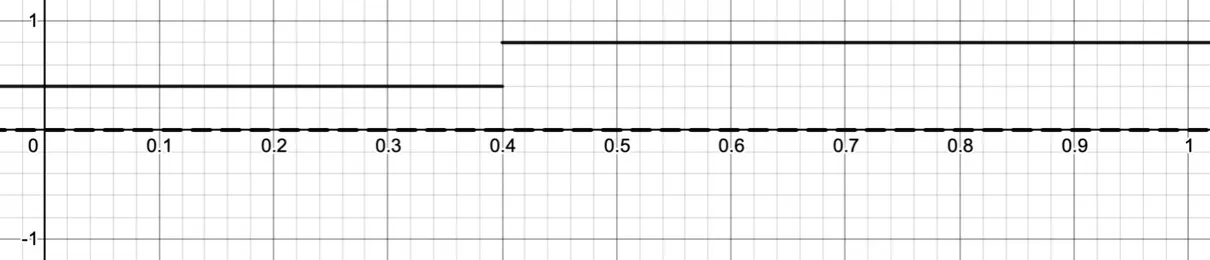
A flat signal has a conceptual frequency of zero (sometimes called “bias” or DC, following the concept of “direct current” in electronics). We can’t hear flat signals, but any non-zero constant should be kept out of audio paths because they effectively change the centerline of an oscillation and limit the available “headroom” between -1.0 and 1.0. But stepped signals are extremely useful for all kinds of control of a patch, as well as for sequencing rhythms and pitch patterns (as we see in Chapter 5).

Whole number (integer) signals

If a signal can only take whole number values, it is considered an integer. You can convert any continuous signal into a whole number signal by passing it through a floor operator (which rounds down), ceil operator (which rounds up), or round operator (which rounds to the nearest whole number). Integer signals can be useful for selecting between modes, picking harmonics frequencies, or quantizing a pitch sequence, etc.

Unipolar logic signals (gate)

Unipolar logic signals are stepped integer signals that can only ever have a value of 1.0 (meaning true/on) or 0.0 (meaning false/off). Here is a logic signal that is “on” for one-tenth of a second and off for four-tenths, etc.

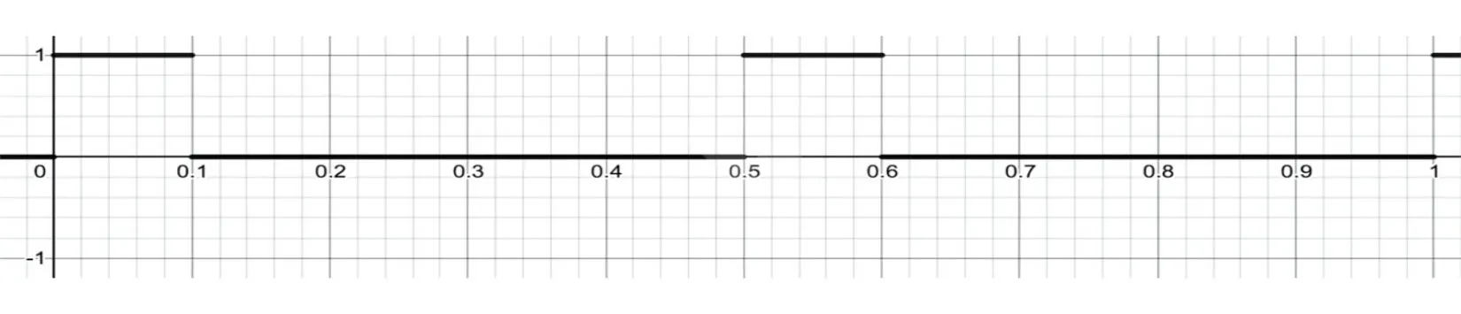
These kinds of signals are produced from the outputs of logic operators, such as < (less than), == (equal)[4], not (logical inversion), and so on. This can be very useful for things like turning other processes on or off.

But for operators with logical inputs, such as the condition input of a switch operator, you can plug in any signal at all, not just zeroes and ones. In these cases, gen~ uses an existential convention in which 0.0 represents a false/off value, and any other non-zero value represents a true/on value.[5]

Bipolar logic (sign) signals

In certain cases, we may want to know the polarity of a signal, which we can get using a sign operator. This is a tri-value logic signal, which is either positive (nominal value of +1.0), negative (nominal value of -1.0), or zero (0.0). Bipolar logic signals can also represent direction without indicating speed: for example, a change operator will give the polarity of a signal’s slope: (+1.0 for rising signals, -1.0 for falling signals, or 0.0 for flat signals).

Single-sample impulse (trigger) signals

This is a special kind of logic signal that is nearly always zero but occasionally spends a single sample frame with a non-zero value, typically 1.0. For example, this graph shows a stream of triggers every tenth of a second, with all other values at zero.

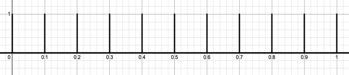
Periodic triggers like this are sometimes called “clock” signals, but in Chapter 2 we will show why we recommend using unipolar ramps for this purpose instead. We use triggers to synchronize the timing of events, starting, stopping, resetting a process, or letting you know the exact sample frame at which some threshold has passed. For example, sending a trigger to the right inlet of a latch operator makes it sample the left input and hold that value at the output until the next trigger.

Stochastic (random) signals

Stochastic or random signals vary over time but without discernible repetitions. The noise operator produces a new evenly distributed random value between -1.0 and +1.0 for every sample frame of passing time.

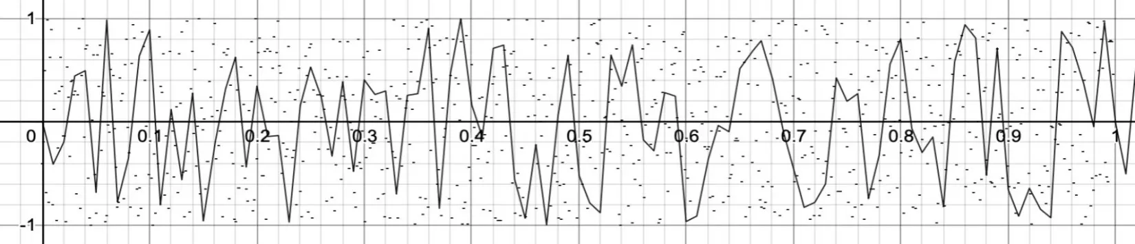
The dotted graph above shows this pure noise, and the solid line shows another stochastic signal derived from noise; these and many other extensions and applications of the unpredictability of chance and chaos are explored in Chapter 4.

A signal can be any of these and something else, too

This isn’t a strict taxonomy. There are no hard and fast rules that define the “differences” between signals — they can be used in many ways at once, carry multiple meanings, or may often morph from one to another. This can be a liberating idea! Here are some examples.

• An envelope isn’t just for shaping amplitude; it could be driving a crossfader or a frequency modulator or anything else

• An audio oscillator can be slowed down to used as an LFO, and vice versa

• A unipolar ramp could be the heart of an LFO, be used to drive a crossfader, determine a tempo-related rhythm, and as you will see in this book, so much more

• A trigger signal could have values other than 1.0, perhaps also being bipolar, to carry more information within it.

• A stream of zeroes could be silent audio, a logical false, an absence of triggers, or just a zero-valued step, etc.

In philosophical terms, all signals have the same flat ontological importance; what’s important is not what they are, but what an operator can do with them. As much as possible therefore we try to design circuits to handle unexpected signal behaviors, such that plugging A into B in an unplanned way may lead to something interesting!

Operators

The gen~ environment provides you with a small number of operators to harness, process, and redirect the flow of signals and, in this way, quickly create complex and efficient patches. They can be divided into a few basic categories.

• Operators that interface with the environment outside (in, out, param, buffer, etc.)

• Operators for fundamental audio signal generation (noise, cycle, etc.)

• Operators for working with ranges of signals (scale, clip, wrap, fold, max, etc.)

• Operators for working with rates or slopes of signals (delta, accum, phasor, etc.)

• Operators for storing data over time (history, latch, delay, data, etc.)

• Routing operators to control signal flows (mix, switch, selector, etc.)

• Math operators such as +, *, pow, sin, round, etc. and logic operators such as and, not, ==, >, etc.

• Operators that perform common numeric conversions (radians, sampstoms, mtof, atodb, etc.), and operators that provide commonly used numbers (pi, sqrt2, etc.) or that relate to the audio engine (samplerate, elapsed, etc.)

• Structural operators for code (expr, codebox) or to embed patches within patches (gen and abstractions)

For some operators, it will be fairly obvious what they do (e.g., a + operator just adds two signals together, and similarly for other math operators such as pow, sin, round, etc), but it might not be immediately clear for many others. Some share names and inspiration with Max and RNBO objects and operators you may be familiar with, though there may also be differences to better fit the gen~ environment.

Aside from the documentation available within Max and online[6], in this book, we’ll introduce and demonstrate different operators as we need them. But first, we’d like to introduce you to a handful of the most frequently used ones. You’ll see these used over and over throughout this book, and understanding how they work and why they’re important will help you develop patches with greater ease.

The param operator

You can use the param operator to add control parameters that you can modify outside your gen~ patch. Each param operator must be named with its first argument, and this name corresponds to messages you can send in the parent patcher to your gen~ object to change that parameter’s value.

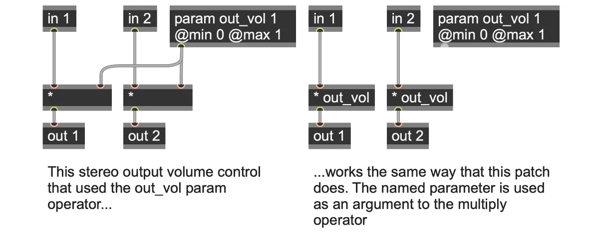
As you can see, you can also use a parameter’s name when performing calculations in other operators within the same gen~ patch. You can also set a param’s initial value with a second argument and limit a param’s range by giving it @min and @max attributes.

Unlike the in and out operators, which allow continuous audio-rate signals into and out of the gen~ patch, the value of a param operator is updated at best at the current signal-vector rate (as defined in Max’s Options: Audio Status window). That is, a param operator outputs a stepped signal.

The history operator (and delay)

Most operators perform work on the value at their input and immediately give the result at their output. The history operator is a little different: it stores the value at its input and outputs it one sample frame later. That means it can function as a single-sample delay. But more importantly–and this is the killer feature–you can route that output through some processing and back to the input in a single-sample feedback loop. This is exactly what is needed to build a multitude of audio processing tasks, including practically all filters[7] and many oscillators, as well as all kinds of nonlinear, chaotic, and cybernetic feedback systems.[8] In fact, many of the other operators in gen~ are really just equivalent to a combination of a history operator and one or more logic or math operators.

You can also give a history operator a name with its first argument, and then it will behave like another param operator. A second argument will set its initial value.

A delay operator is like a series of many history operators in series that you fill one sample at a time and read values out at different delay times. Like the history operator, it also lets you patch feedback loops, and we’ll look at this in depth in Chapter 7.

The scale operator

We talked earlier about thinking of a signal’s range of values. Frequently, we need to map a signal from one range of values to a different range of values[9], and the easiest way is to use the scale operator. All you need to know is a pair of corresponding points. For example, you could create a Fahrenheit to Celsius converter using scale 32 212 0 100, since the freezing and boiling points of water are 32° F and 212° F respectively at the input, corresponding to 0° C and 100° C at the output.

Here are some more relevant examples that we very frequently use in this book:

• To convert a bipolar normalized signal (-1.0 to +1.0) to a unipolar normalized signal (0.0 to +1.0), use scale -1 1 0 1. To convert the other way, just reverse the inputs and outputs: scale 0 1 -1 1.

• To turn a unipolar signal upside down (which is also called inverting it), we can pass it through a scale 0 1 1 0 operator.

For a more involved example: A modular synthesizers sometimes use a convention to represent pitch called “volt per octave” where increasing a value by +1.0 means going up by one octave, which is the same as going up 12 semitones in MIDI note numbers. If our reference value of 1.0 corresponds to MIDI note number 24 (note C1), then a value of 2.0 indicates MIDI note number 24 + 12 = 36 (note C2), and we can use a scale 1 2 24 36 operator.

A scale operator with no arguments will have a series of additional inlets to dynamically set the input and output ranges with input signals (defaulting to 0.0 to 1.0 ranges if not connected).

The wrap, fold, and clip operators

These operators are all useful ways to set limits or boundaries of a signal in their left inlet. You set the lower and upper bounds in the operator’s arguments or other inlets, and any input value that is outside these bounds will be transformed so that it remains within them.

With the wrap operator, any value that exceeds the upper bound will automatically wrap back to the lower bound value, and vice versa. This creates a kind of circular number space, a bit like the way an angle of 365° is the same as an angle of 5°, or that 13:00 is the same as 1pm.

This turns out to be incredibly useful, and we’ll see it in many forms in this book.

• Creating a ramp oscillator from a history, a +, and a wrap operator

• Building modular arithmetic for tempo manipulations and Euclidean rhythms

• Operating on musical pitch spaces

• Pulling out the fractional part of a number for interpolation purposes

The wrap operator has several close relatives that differ in handling out-of-range inputs. The fold operator reflects any signals outside the range back in, whereas the clip operator (also known as clamp) holds the value at the limit. So, for example, if the input signal is 1.2, a clip 0 1 operator would output 1.0, a fold 0 1 operator would output 0.8, and a wrap 0 1 operator would output 0.2.

The accum (and phasor) operators

The accum operator (also known as the += operator) can be used whenever you want to keep a running count. If you send it a signal of occasional triggers of 1.0, it will count how many triggers it received. If you send it a constant signal of 1.0, it will add one for every passing sample frame and thus count how many sample frames have elapsed. But the accum operator doesn’t have just to count in ones, it can add up any input values at all. (In mathematical terms, it performs stepwise integration.) It can also reset its count to zero whenever its right inlet receives a non-zero signal. You can use the accum operator for many useful things.

• Measure elapsed time (in whole number samples or other units of time)

• Index samples for playback from an audio buffer

• Build slope generators for envelopes and other modulations

• Combine with a history and wrap operator to create a cycling phasor

A phasor operator is another accumulator that counts in tiny increments from 0.0 to 1.0 over and over, creating the kinds of repeating ramp signals we use at the core of oscillators and rhythms, as we will see in Chapter 2.

The delta (and change) operators

We noted earlier how important it is to think about the rates of changes of signals. The delta operator tells you how much a signal changes in value from one sample frame to the next, whether positively or negatively. To take an analogy from physics, if the signal represents a position, then the delta gives you the velocity. (This is like the stepwise differentiation of calculus: it is the difference quotient of the signal per sample frame. In that sense, it’s the opposite of the accum operator!)

It’s really just the input minus the previous input, which provides you with the slope of a signal. This deceptively simple slope-per-sample measurement lets you do some amazing things.

• You can use the magnitude (absolute value) of a delta operator’s output (or a filtered version of it) for things like onset detection in waveform processing.

• When a delta operator is combined with a wrap -0.5 0.5 operator, you can get the slope of a phasor ramp without “jumps.” And from that, you can derive the phasor’s frequency and many other features, as we explore in Chapter 2.

• Connecting two delta operators together lets you detect kinks and curves in an input signal: the rate of change of the rate of change, or acceleration of the signal.

• The sign of the delta operator’s output is a bipolar logic value that tells you whether an input is rising (sign = 1), falling (sign = -1), or staying the same (sign = 0). This is also exactly what the change operator does.

• Chaining two change operators together will give you a bipolar trigger when a signal switches direction, picking out only its peaks and troughs.

The latch operator

The history operator lets you hold a value from one sample frame’s worth of calculations to the next, but it then immediately forgets it because signals are always flowing through it. If you want to hold on to a value for longer and only let it update when you say so, you want a latch operator.

The right inlet expects a trigger or logical control signal to activate the latch. A non-zero trigger at this inlet will “sample” the left inlet’s value, passing it through to the outlet. A zero value at this inlet means that the previously sampled value will continue to be held and output. This behavior is often called “sample and hold.”

However, suppose the signal at the right inlet is a logic signal rather than a trigger. In that case, any non-zero value (meaning “on”) at the latch operator’s right inlet will let signals pass from the left inlet right through to the outlet. Still, with a zero at the right inlet (meaning “off”), the latch operator will keep outputting the previous value, effectively freezing the signal. This is sometimes called a “track and hold” operation.

The latch operator’s simplicity belies its usefulness. Here are some examples.

• If you feed the control input a trigger signal, the output will be a stepped control signal. In this way, you can slow down the rate of change of a process, which can be handy in bringing fast changes down to human-readable time frames.

• A triggered latch operator can also be used to synchronize one process to another, such as updating a process parameter only when it has been cross faded out or holding parameters constant throughout a grain’s envelope.

• A set of interconnected latch and history operators can form the basis of a “shift register,” which we use in several places in this book, including creating smoothed random signal generators in Chapter 4 and building algorithmic sequencers in Chapter 5.

The mix (and switch) operators

As you might guess, you can use the mix operator to crossfade between two signals. Send a unipolar (0.0 to 1.0) signal in the right “mix” inlet to crossfade from the left inlet (with the mix at 0.0) to the middle inlet (with the mix at 1.0) or any blended point in between. But don’t let your imagination stop at crossfading audio signals. There’s a world of interesting things we’ll do throughout this book with mix operators.

• A mix and a history operator in a feedback loop will give you a running average, which you can use to smooth out stepped signals, or to lowpass filter audio,

• You can also use it to find weighted averages between data points and, with a couple of latch operators and a phasor, create a sequence of ramp segments,

• You can use a mix operator as a linear interpolator between points, such as mixing smoothly between quantized values (and possibly with different curves),

• We will also see the mix operator used to compute sub-sample waveform points for antialiased (band-limited) oscillators!

If you don’t need to crossfade and just want to switch between two inputs, you can use the switch operator (also known as the ? operator). The switch operator performs basic logic if-then-else routing: if the left input is true (any non-zero value), then it passes the middle inlet through; else, it passes the right inlet through.

The buffer and data operators

These two operators let you work with stored collections of sequential values, such as from audio files, which can either be mono or multi-channel.

A buffer operator in gen~ lets you access the data of a regular buffer~ object in the parent Max or RNBO patch. You do this by giving them the same name (the first argument). The underlying data is shared: if you write to the buffer in gen~, it will also be changed in parent’s buffer~, and vice versa; if you load a new audio file into the buffer~ in Max, the buffer in gen~ will also change.

In contrast, a data operator’s storage is local, meaning it belongs only to the gen~ patch and cannot be accessed from outside. You must give the data operator a name and declare its length (and optionally also specify the number of channels). The data operator is like a collection of history operators in parallel, which you can read from and write to however you like.

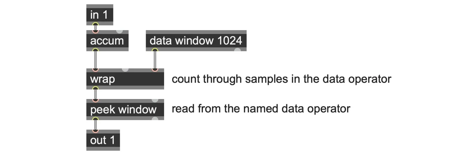
The buffer and data operators don’t do any signal operations themselves; they just output their total length in samples and their number of channels. To write a value to a buffer or data, use a poke operator with a matching name argument, and set the new value and sample position via its inlets.

To read values from a buffer or data, use peek or sample operators with matching name arguments and send them a sample position (for peek) or a 0.0 to 1.0 phase (for sample) at the inlet. We’ll see peek and sample in the next chapter and go into them much more detail in Chapter 9.

The codebox operator

Gen~ is primarily a visual programming environment, but it also offers a way to write algorithms with text-based code when you want to, using a simple language called GenExpr within codebox operators. You’ll the codebox used for patches in this book from time to time, but we use it sparingly and only when it’s necessary for the tasks we’re working on. Here are some of the reasons that we usually prefer visual to textual programming.

• You can place comments anywhere and lay out the algorithm spatially to convey what it does, add assistance comments on in and out operators, etc. This means the patch can be easier to understand when you return to it months later and make more sense to others when you share it.

• You can make more efficient use of reference resources (by Option-clicking [Macintosh] or alt-clicking [Windows] the operators, or using the reference sidebar)

• Errors in textual code are much easier to make, harder to understand, and can break your workflow. It’s almost impossible to make a syntax error with visual patching.

• Using a codebox operator does not make your patch any more efficient.

The last point may surprise some readers, as there seems to be some mystique among the community to the contrary. There is absolutely no difference in terms of performance between using visual patching compared to utilizing a codebox operator to do the same thing. The gen~ environment always converts all the visual patching into GenExpr anyway (and you can see that GenExpr code by looking into the sidebar of the patch marked with a C symbol). Everything in the patch–whether it be visual patching or codebox operators–gets merged into a single representation. The gen~ environment then uses that representation to generate and compile fast native code on-the-fly.

On the other hand, there are a few situations where there are very good reasons for using a codebox operator in your patch, and you’ll see us using a codebox in these situations:

• If you had done textual coding first, then on your first encounter with visual programming you might have asked, “how do I write an if/else or a for loop?” The codebox operator is necessary if you need to perform procedural branching and looping with if(), for(), or while(). It’s the only way to include those kinds of procedural operations. However, it can still be better to avoid using these if you can.[10]

• The codebox operator gives you precise control of the order of reads and writes for working with delays and operations on data and buffer operators. While you can mostly achieve this with visual patching, there will be some cases where you want to lay out a specific order for these operations, and a codebox operator may be your best choice.

• Using a codebox might make it easier to translate some other code or a math expression found “in the wild” into the context of your patch.

The gen operator (and abstractions)

If you have a sequence of operators that achieve a single task together, grouping them into a subpatch (a patch within your patch) can make sense. Within a gen~ patcher we can use a gen operator to create a subpatch–just double-click the gen operator to open and edit it. Within the subpatch, you can use the in and out operators to create inlets and outlets of the gen operator. Encapsulating bits of patching into a gen subpatch can be a great way to organize your patches for clarity. We recommend you also give the gen operator a @title attribute to remind you what it does when you return to it later!

But what if you created a patch that does things that would be useful in other patches? Any handy gen~ patch (or subpatch) can be saved to an external file using Save As… from the File menu, which saves the patch as a .gendsp format file. These .gendsp files can then be reused as “abstractions” in other gen~ patching contexts just by typing their name into a new operator box as if they were just another gen operator. This means you’re not limited to the set of operators provided. Building up a library of handily reusable abstractions allows you to design your own set of tools with the needed features.[11]

The “go” library

Throughout this book, we frequently solve problems with bits of patching made of a handful of operators, and we have saved these as reusable abstractions. These abstractions are all named with the prefix “go.” (from “generating” and “organizing…” in the book’s title[12]), and you can find them in the “patches” folder of the software that accompanies this book.

If you have placed the software in your Max package folder, you’ll be able to use these “go” anywhere you want to. They provide subcircuits for common tasks for working with signals, including shaping them, detecting specific changes or other logic, generating complex control sources, applying filters to audio, and other starting points for higher-level patch functionality. For example, the go.ramp2trig.gendsp abstraction outputs a trigger signal that spikes whenever an input ramp signal completes its cycle, which is something we need very often! You can add one to a gen~ patch simply by creating a new operator named go.ramp2trig. We’ll build this abstraction and use it extensively in the next chapter.