Chapter 7:
The Effects of Delay

Repetition is the mirror of the infinite, and working with delay is like traveling through time, which can get a little mind-bending — especially when feedback is involved. It may be helpful to approach the subject in terms of analogy. Consider a tape loop:

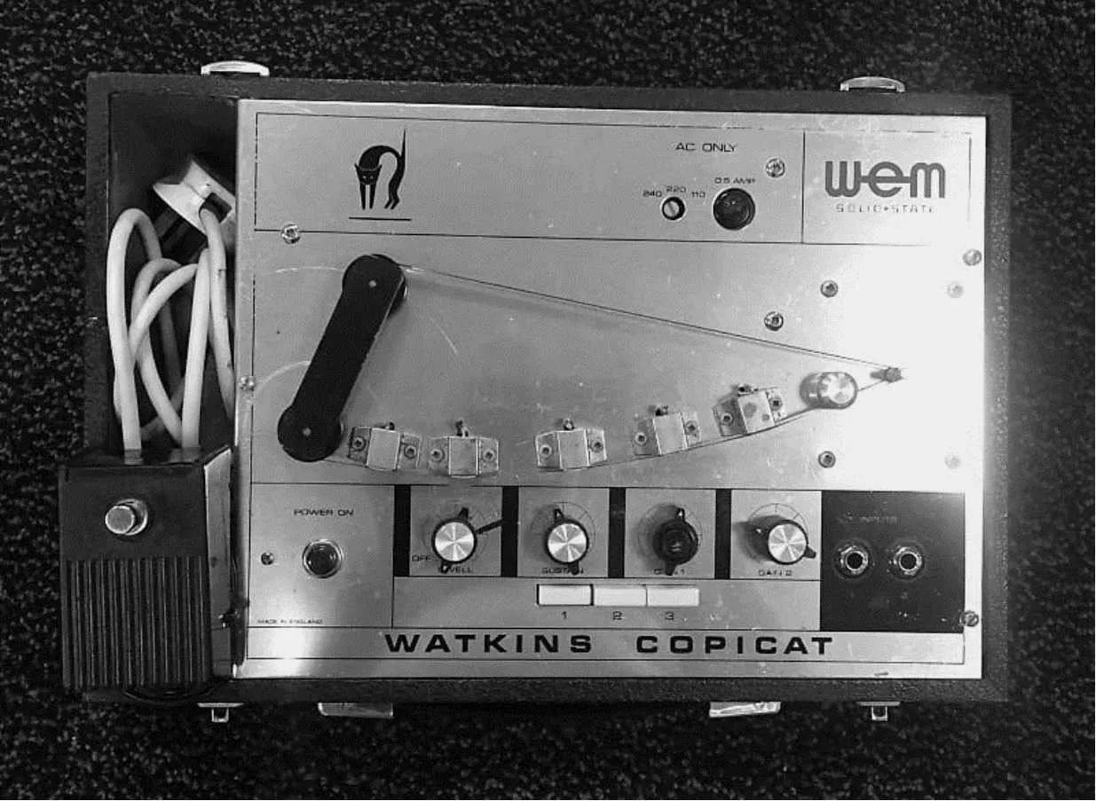
Watkins Copicat photo courtesy of Mike Podest

A basic tape loop has three kinds of “heads,” which just means points where information goes in or comes out of the tape:

A write head	One or more read heads	An erase head

These heads can be positioned anywhere on the tape loop as the tape passes through them at a steady rate. The distance between the read and write head determines the length of the delay. The delay corresponds to the time between the moment a signal goes into the tape at the write head and the moment when that same bit of tape comes through the read head and the signal is read out. A larger distance between a read head and the write head results in a longer delay.

A “multitap delay” has several read heads—one for each “tap”—usually located in different positions, corresponding to different delay times. The tape stores data written in the past, and each reader picks a different distance in the past to read from.

The eraser head is usually located right before the write head so that new sounds can replace the sounds already on the tape. (Or, if the erase head is disengaged from the tape, then new sounds will overdub or mix with sounds already on the tape for layering sound on sound loops.)

A basic delay loop

A digital delay is similar to having a tape delay, but the physical tape is replaced with an array of sample slots in digital memory.

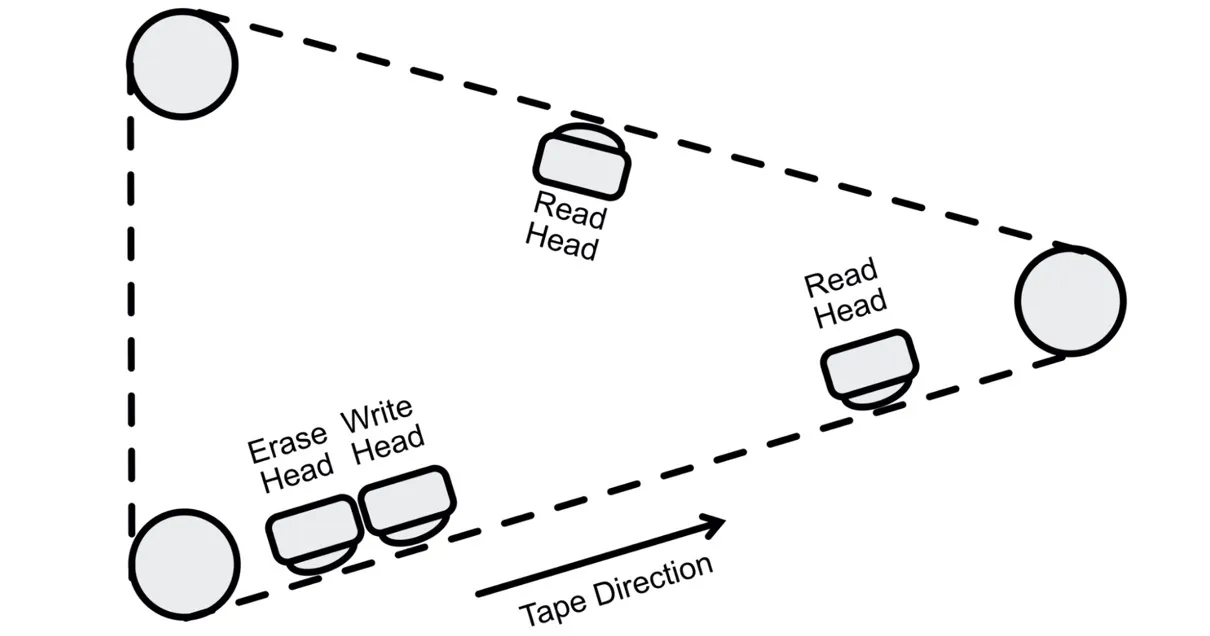
Here is what that means.

• The tape loop is always moving at a constant rate, corresponding to the current sample rate. The tape is thus “ticking” through in discrete steps at thousands of times per second.

• Every new input at the “write head” fills the next sample slot in the array of samples (the “tape”).

• The delay time sets how far back in this tape the “read head” looks to fetch its next output.

In gen~, we can do this using the delay operator. This operator can take two arguments:

1. The first argument defines the maximum possible delay time in samples and thus the amount of memory to be allocated. In effect, it specifies the length of the “tape loop.” If you don’t specify this length, it will default to one second at the current sample rate.

2. The second argument sets the number of read heads (or “taps”). The default is 1 (a single tap). The number of taps specified in the argument will determine the number of inlets and outlets the delay operator will have.

The first inlet to the delay operator sends audio to the write head. Additional inlets set the positions of the other read heads (taps) in sample frames, which means their distance from the write head. The outlet(s) are what these read heads read from the tape. (The eraser head is inside the delay, sitting right before the write head).

Here’s an example of the delay operator in use:[63]

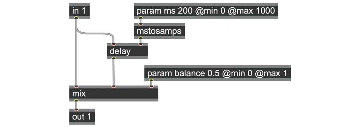
delay_feedforward_basic.maxpat

We set the delay time in terms of samples since that’s what the tape itself uses. We can use the mstosamps operator to handle conversion from milliseconds for us. In the patch above, we also added a mix operator to let us blend the wet (delayed) and dry (original) outputs so that we can hear a blend of both.

Feedback

The previous patch is called a “feedforward” delay because the output of the delay feeds forward to the output of the patch. But we can also create delays that “feed back” upon themselves, creating a feedback loop. So far, we’ve only patched feedback loops in gen~ using the history operator, but the delay operator can do this too.[64]

So, we could simply take our mixed output and feed the result back into the delay.

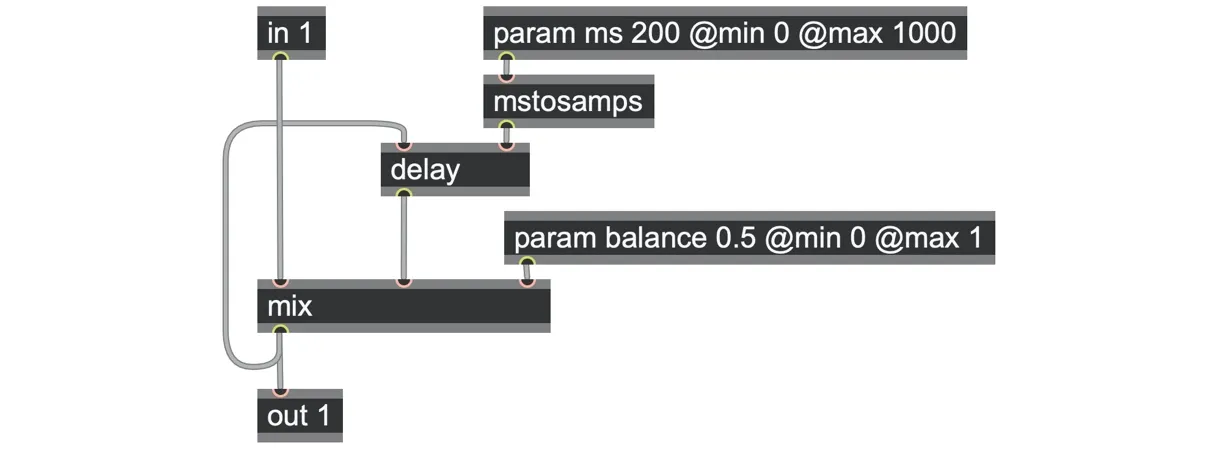
delay_feedback_basic.maxpat

You might notice that this bears a striking resemblance to the basic one-pole filter example we built using mix and history operators in Chapter 6, but with the history replaced by a delay. That is, the feedback delay is just a one-pole filter stretched out in time! (We'll see later in this chapter that you can also turn other filter structures into interesting delay effects by replacing history operators with delay operators).

Try playing a sound through this patch. Set the balance to 0.5 and delay time to 200 milliseconds for a classic echo sound. Now, turn the balance up to 1.0, and the sound will appear to freeze into a loop. At this point, we only hear the recirculating “tape.” Set the balance to around 0.97, and the captured loop will slowly fade away again.

If you wanted to separate the control of the wet/dry balance from control over the amount of feedback, it could look like the following patch. We marked the signal feedback loop clearly in a darker color to identify it.

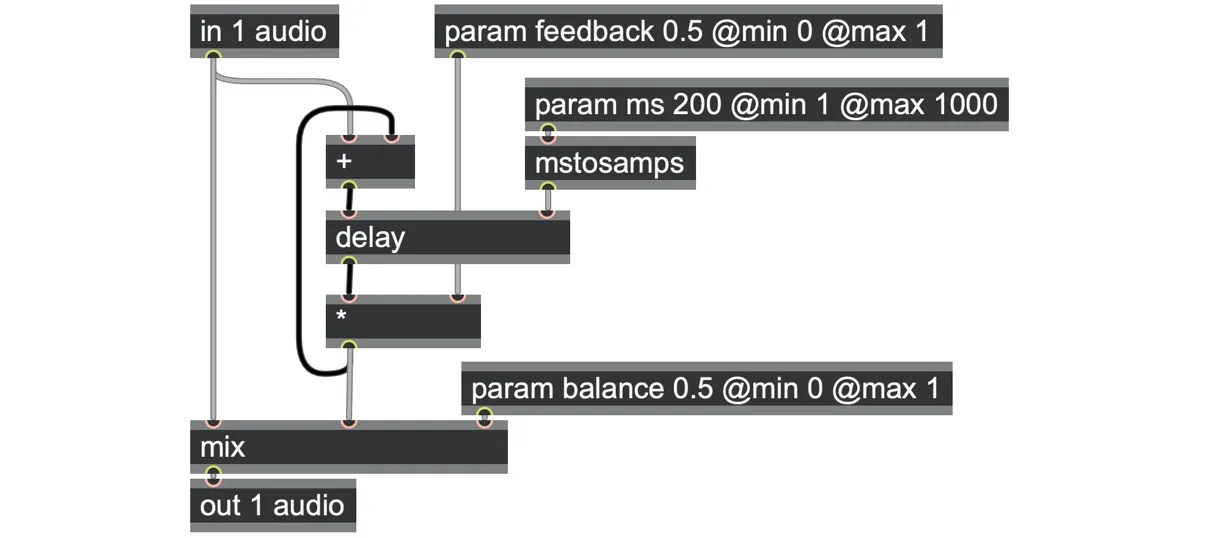
delay_feedback_basic.maxpat

Watch out, however — setting the feedback to 1.0 can start to overflow since the input is still being fed into the delay (meaning that nothing is ever lost), like trying to squash more and more stuff into a bag; we will return to the issues this can cause a little later.

Setting the feedback decay time

You might notice that a delay-based feedback loop fades away more quickly when the delay time is short and more slowly when the delay time is long. It makes sense: the shorter the loop is, the more often the feedback multiplication is applied to a given sound, so the more quickly it shrinks. How can we ensure that a delay effect will decay over a specific amount of time, regardless of the delay time setting? Just as we used the t60 operator in Chapter 6 to determine filter response times, we can also use it here to determine a delay's decay times.

It helps to think of the t60 value as a multiplication per feedback loop. In a history loop, the feedback is just one sample long, so there’s multiplication at every sample frame of real-time. In a delay tape loop of 10 samples’ length, the feedback multiplication applies to a specific step in the tape loop only once every 10 sample frames of real-time since it takes that long for the “tape” to loop around. That’s just 1/10th as often.

So, to compute the feedback multiplier for any feedback delay, we divide the desired decay time (in samples) by the delay length (in samples) and feed that into the t60 operator, as shown in the following patch. The echoes will now decay over the same amount of time (param decay_ms) regardless of how long or short the tape is.

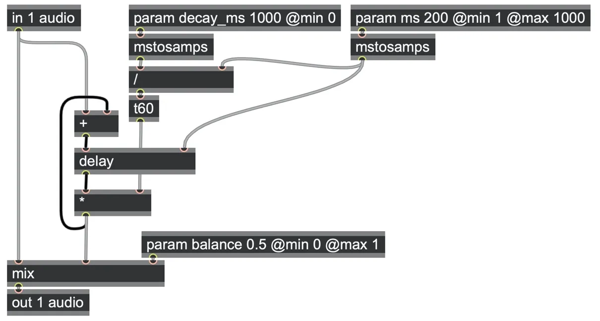
delay_feedback_decaytime.maxpat

Feedback filtering

Most physical echoes don’t just get quieter over time. They also get duller as the physical objects that echoes reflect off absorb higher frequency energy with each bounce. We can easily emulate this by placing a lowpass filter into the delay feedback loop. However, we should be careful not to use a resonating filter that would increase energy at any frequency, or the sound could blow up! Here we can reuse the go.onepole abstraction we built in Chapter 6 as a non-resonating filter placed in the feedback loop.

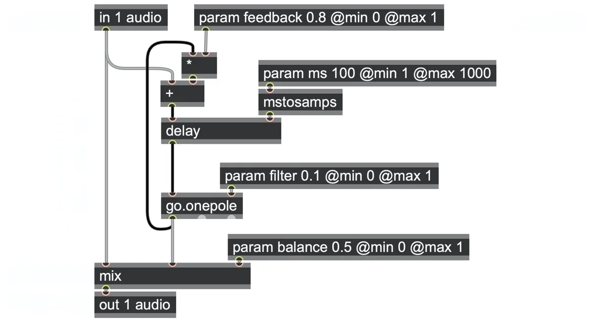
delay_feedback_filtered.maxpat

Removing DC

If you set the feedback parameter to 1.0 for infinite repeats and keep feeding a signal into the delay, you might notice that with some inputs the delay output waveform begins to drift away from the center zero line (for example, try looping the anton.aif sound file).

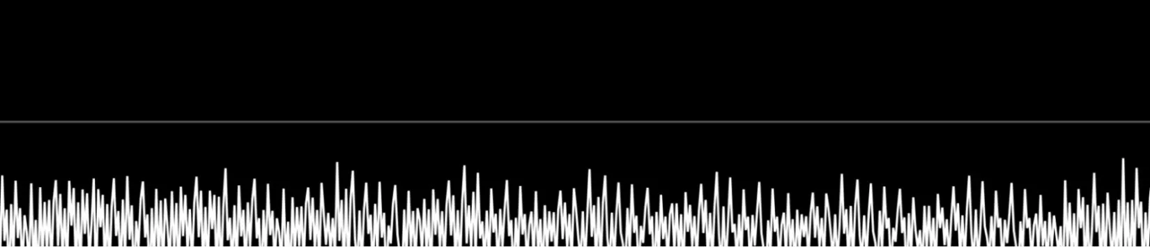
What’s happening is that the average value of the input sound’s average is not quite aligned to zero, and this small deviation is being added each time through the feedback loop. This recirculated drift can accumulate to the point that the signal entirely wanders beyond the acceptable bounds of -1.0 to +1.0 and begins to clip and distort. The shift away from the zero point you see here as an electronic average is known as DC (direct current) or near-zero frequency energy. We can eliminate this problem by use of a “DC-blocking trap,” which is simply a highpass filter with a cutoff frequency below the audible range. This will drain away accumulated deviations from the zero line without affecting the frequencies we can hear.

For example, we can use the second (highpass) outlet of the go.onepole.hz abstraction that we built in Chapter 6 set to a sub-audible cutoff frequency of 3Hz. Here, we put this on the input to the delay so that it will also reduce DC before it even gets a chance to enter the delay loop.

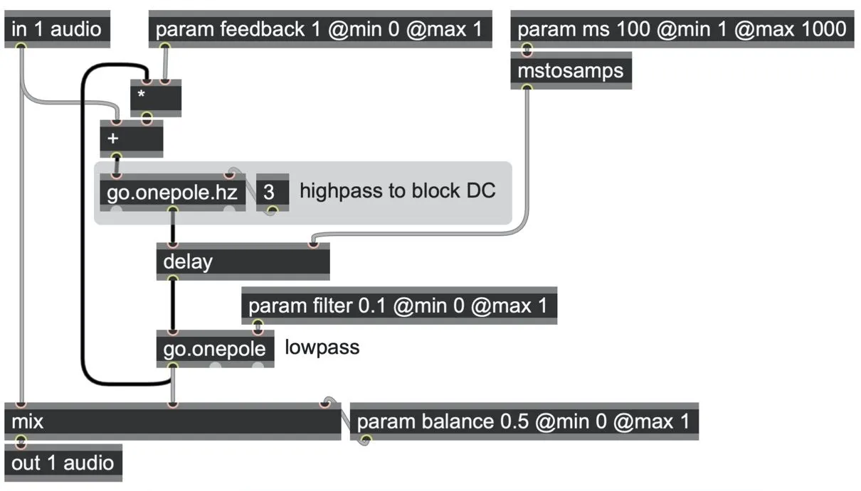
delay_feedback_filtered_dcblock.maxpat

Feedback limiting

Accumulating DC isn’t the only thing that can go wrong with a feedback loop. Another is simply the accumulation of too much energy overall, especially if our feedback parameter is set high or we have a resonant filter in the loop. More generally, for any feedback system, we may end up producing positive feedback (in which the energy recirculating in the system is amplified) that can very quickly blow up into exponentially large signals.

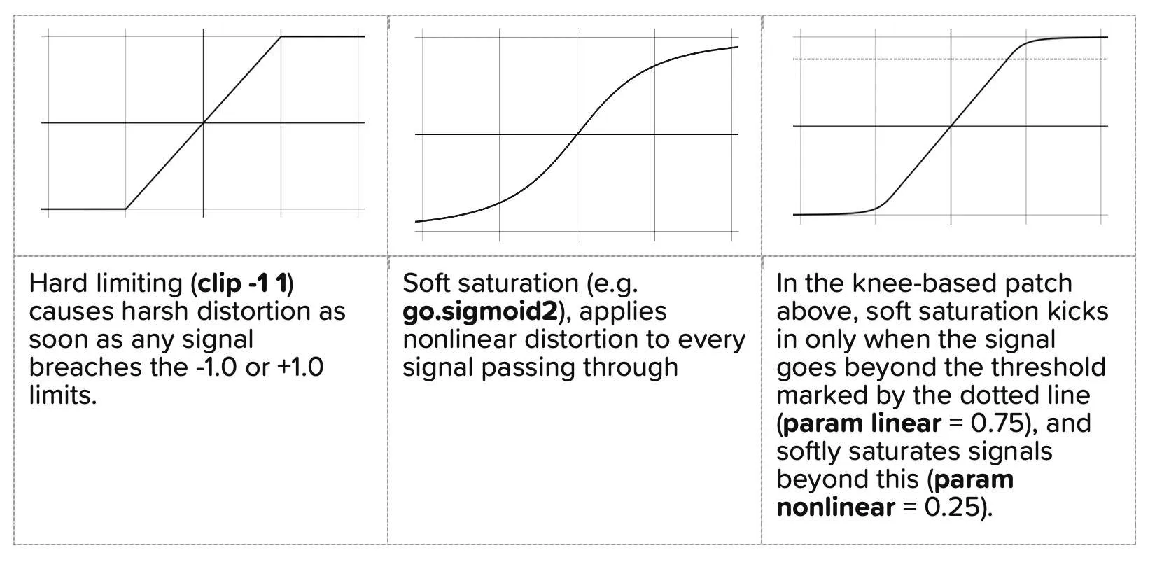
One strategy we can take here is to apply some kind of limiting process, such as hard clipping with a clip -1 1 operator such that positive feedback cannot go beyond the safe -1.0 and +1.0 limits; however, this sharp cut will add very harsh distortion to any signal that does.

Alternatively, we could use a soft saturator, including any of the sigmoid functions we encountered in Chapter 3 within the feedback loop, such as a go.sigmoid2 abstraction. These will also ensure that no matter how much the signal gains positive feedback, the output remains between the safe -1.0 and +1.0 limits, and instead of the harsh distortion of the clip operator, they will impart a softer and more pleasant harmonic distortion. The delay_feedback_saturated.maxpat patch shows an example of combining a resonant bandpass filter with sigmoid waveshaping distortion, evoking a classic space echo dub delay effect.

As nice as this distortion can be, it will change the sound of any signal going through it, regardless of whether it is excessively loud or not. If we didn’t want the saturation to influence the sound this much, we could apply a pragmatic solution: up to a certain threshold (sometimes called the “knee”), we can pass through the signal unchanged. Beyond this threshold, we can apply the nonlinear distortion, scaled such that it squishes the remainder to a more limited range.

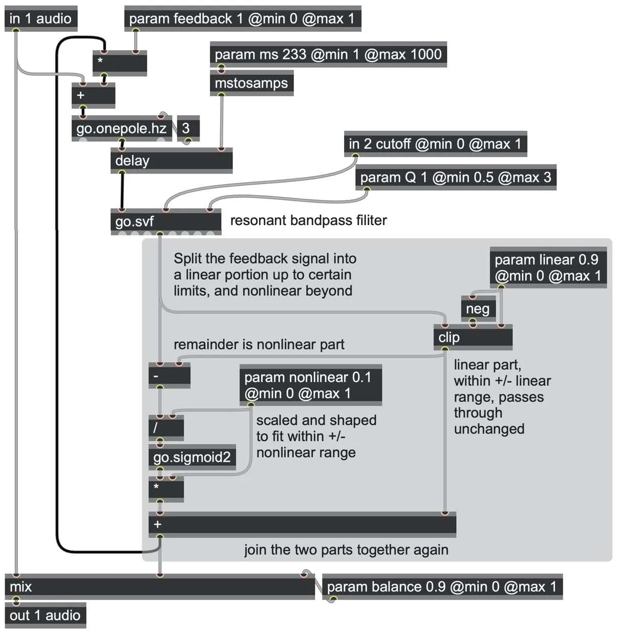
delay_feedback_saturated.maxpat

Up to the param linear threshold, the signal passes through unchanged, while the remainder of the signal beyond this threshold is squished to fit within the param nonlinear range. In this way, the final output amplitude cannot be greater than linear + nonlinear.

Here are these three approaches compared graphically, in which the horizontal axis represents the input amplitude, and the vertical axis is the output amplitude

Avoiding clicks

You’ll probably notice that changing balance and feedback parameters can sometimes cause clicks in the output. It makes sense when you think about it. If you scroll values in a Max or RNBO number box, param attrui, or any user interface that is updated lower than audio sample rate, the value will be stepping in short jumps. Since these parameters are being used to multiply an audio signal, it is like making an instantaneous “jump” of a volume fader, which would result in a click.

This can be fixed by adding parameter smoothing—turning a sudden change into something more gradual. We could reuse the go.line.ms lag generator we built in Chapter 7, or a one pole or slew limiter, to ensure that all parameter changes are smoothed over a period of time, as shown in the following patch. The amount of ramp time we need doesn’t have to be very much — a handful of milliseconds or a couple of hundred samples is usually enough to remove the clicks.

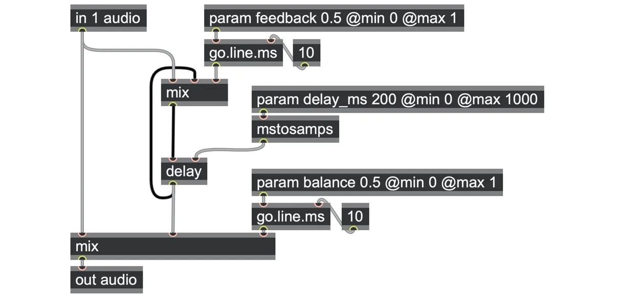
delay_param_smoothed.maxpat

When you twiddle the delay_ms parameter, it can also create artifacts, but this happens for a different reason. If the delay is like a tape of sample frames, then a sudden change of the delay time parameter is instantaneously like teleporting the read head from one position on the tape to an entirely different position on the tape. That's very likely to cause a click because the waveforms at two different locations are likely to be quite different, causing a sudden jump in the output. We'll look at two possible solutions for this next.

Smooth changes to delay time cause Doppler shifts

What if we were to use parameter smoothing for the delay time too? Then our read head will not be teleporting but will be moving gradually and continuously back and forth around the tape: each jump is now so small that it doesn't cause glitches.

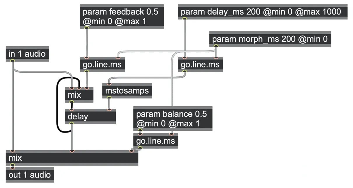
delay_morphed_times.maxpat

Instead, this gradual change of delay time ends up creating a pitch-changing effect. Here, we spread the ramp over 200ms to make the effect more visible:

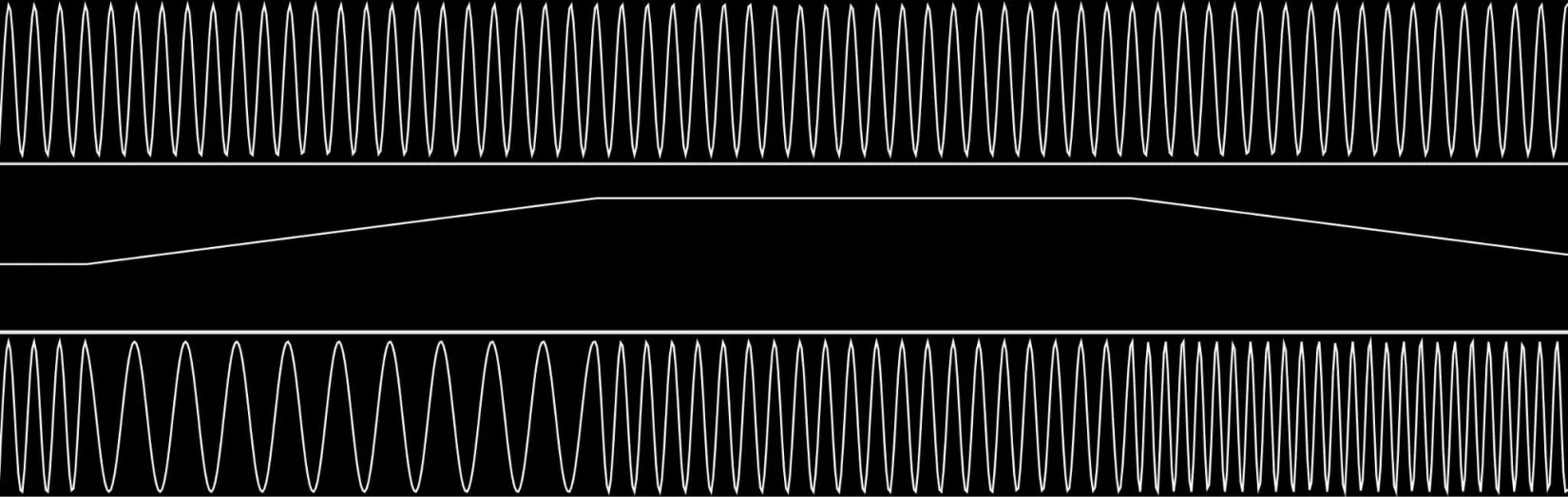
Top trace: Sine wave input at 100Hz. Middle trace: the delay time (ramping up and down between 100ms and 200ms). Bottom trace: the delayed sine wave. Notice how the sine wave is stretched out (pitched down) as delay times increase and is compressed (pitched up) while delay times decrease.

The pitch change is due to relativity. Increasing the delay time is like moving the read head away from the write head, which, relativistically speaking, is the same as if the tape were playing more slowly–from the point of view of the read head. Some digital instrument designers call this “analog-style delay” since it mimics what happens when you move heads on physical tape delays, but it is also equivalent to the Doppler shift of a fast-moving object in space. Moving a sound source and listener apart (increasing delay time) will effectively stretch the traveling wavefronts out (lowering the frequency) while moving them closer together will compress the traveling wavefronts (which raises the frequency).

Suppose you want to know precisely what the pitch change will be for any delay time modulation. In that case, you can send the delay time parameter through a mstosamps operator to convert it to sample frames first, then get the slope with a delta operator. This gives you a positive value when the delay time is increasing, negative when it is decreasing, and will be zero when the delay time is not changing. If you subtract that from 1.0 using a !- 1 operator it will return a value of 1.0 when the delay time is not changing, a value of 2.0 when the delay time modulation causes the sound to double in frequency, a value of 0.5 when the delay modulation causes the frequency to halve, and so on.

We can turn this into an octave pitch signal by passing it through a log2 operator for the exponential pitch space and a go.octave2midi abstraction if we want MIDI pitch offsets.

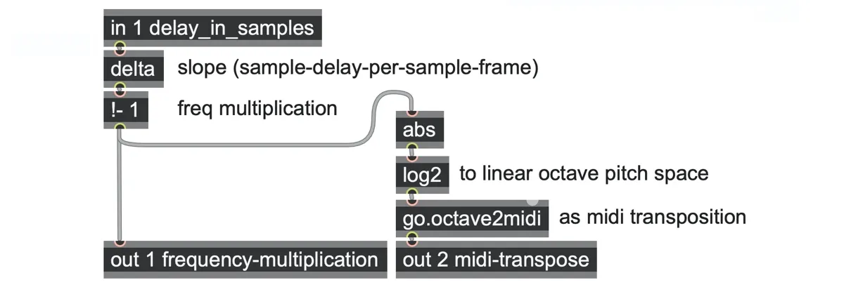
Conversely, we can reverse this calculation to modulate a delay for a desired pitch change: from an octave pitch signal, apply the exp2 operator to get back to the linear frequency multiplier, add + 1 for the base multiplier, and feed that into an accum operator to integrate the required variable delay time in samples. Both of these transformations are demonstrated in the delay_morphed_times.maxpat patch. Now you can play a Doppler melody on any sound input!

Changing delay time without pitch shift

If we want to change delay times without causing clicks and also without causing any pitch shifting, we can resort to a little sleight of hand. We’ll run two taps–let’s call them tap A and tap B–and we use a mix crossfader so that normally only one of the taps is being heard. If the mix factor is 0.0, we only hear tap A, so we can freely change the delay time of tap B without clicks. If the mix factor is 1.0, we only hear tap B, so we can freely change tap A. (You could think of this as a bit like a DJ flipping the crossfader over to deck B in order to rewind the track on deck A, then crossfading back.) The crossfade can be just a few milliseconds long — just long enough to soften any sudden change in the waveform. In the following patch, we use a go.line.ms abstraction to perform the crossfade over 12 milliseconds.

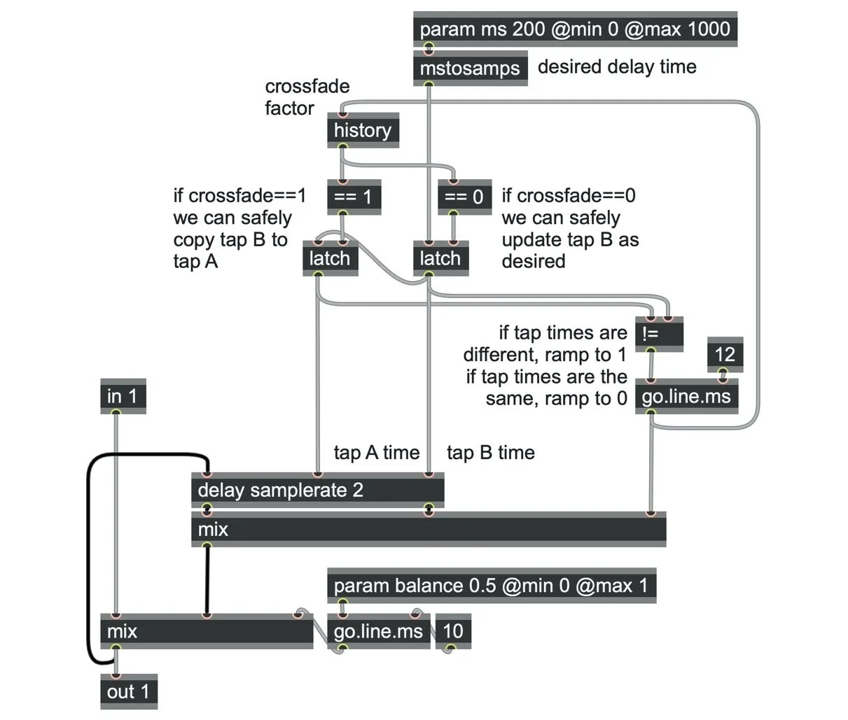
delay_morphed_times_no_pitch_change.maxpat

This crossfader value (stored in the history at the top right) acts as a kind of state machine that drives the whole patch. The states are either

• A value of 0.0 (listening to tap A)

• A value of 1.0 (listening to tap B)

• A value in transition somewhere in between (hearing the crossfade)

That bit of patching is quite a useful little combination, and we’ll use it again later, so we saved it as go.background.change.gendsp.

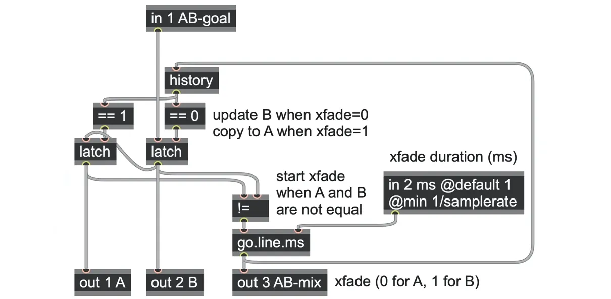
go.background.change.gendsp

A garden of earthly delays

So far, we have been looking at delays as a way to create echoes or periodically repeat input sounds with a time offset, but there is a much broader range of well-known and beloved audio effects made possible by delay operations at shorter time scales, including chorusing, flanging, voice doubling and so on. The main differences lie in the range of the delay times used and how they are modulated and mixed—many of them also employ some kind of low frequency (LFO) modulation of the delay time.[65]

In fact, we can create a single patch combining some of the ideas we’ve seen so far in this chapter that can be used to reproduce many different delay-based effects by simply varying its parameters.

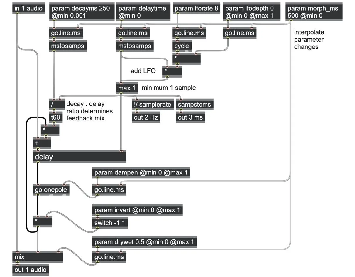
delay_multi_effect.maxpat

This patch combines a delay with a feedback loop using the t60 operator to set the total decay time and a go.onepole abstraction to apply filtering to the feedback, as we have seen earlier in this chapter. In addition, the param invert adds the ability to multiply the signal by -1 each time through the feedback loop. But probably the most important addition is the ability to modulate the delay time with an LFO whose rate is set by the param lforate operator and the intensity of its effect by the param lfodepth operator. Most of the parameters are fed through go.line.ms abstractions to smoothen their changes.

Here is a list of example parameter settings and the very different sonic effects they can have listed in order of delay time.

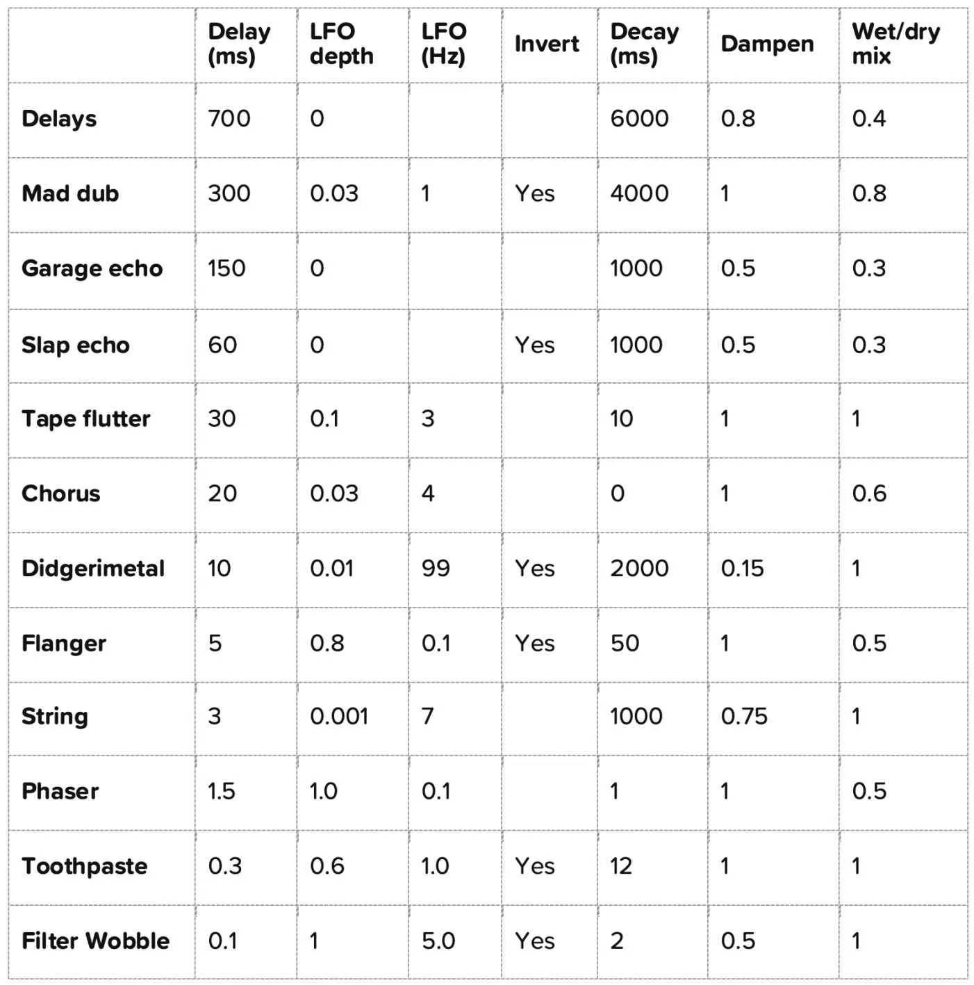
You can select and morph between these using the umenu interface in the delay_multi_effect.maxpat patch. It’s worth spending some time trying out different input sounds and testing and listening to the output to get a sense of these effects and how their parameters interact. Some of these are well-known “classic” effects; others are a bit more experimental. You may also find it interesting to set a high param morph_ms value to listen to the intermediate sounds as the patch “morph” between these examples.

We think it is quite amazing how many different sonic results can come from a fairly simple patch. Let’s look at some of them more closely, working our way down from echoes to the microsonic realm of filters.

We hear clear individual repetitions with longer delay times of around 100ms to one second or more. Without feedback, this can seem like musical hocketing; with lots of feedback, it can produce a sensation of rhythm or tempo.

Slightly shorter delay times resemble tape-head or slapback echoes associated with devices such as the Watkins Copicat, whose image opened this chapter, and adding a little judicious LFO modulation can introduce some “tape flutter.” Delays in the 20-100ms range with feedback can begin to fuse into trill-like trails, perhaps reminiscent of room echo, and adding some damping filtering will make them sound less metallic.

Below this range, we no longer hear individual repetitions, and the rhythmic effects turn into effects that we identify by their spectral content. As the delay time is shortened to around 10 - 30ms, a blend of dry and delayed sounds can appear to reinforce themselves (commonly referred to as “doubling”) and add a slight amount of modulation to the delayed signal to introduce subtle changes in pitch will lead to characteristic “chorus” effects. Chorusing is similar to vibrato because it introduces subtle changes in pitch by modulating the delay time with an LFO. Varying the rate of the LFO will generate more phase shift (and perceived pitch modulations) of the original signal.

The span of 0.5 - 25ms corresponds to the realm typical of musical pitches (from 2000Hz down to 40Hz, respectively). If we set the feedback very high and feed the delay with bursts of noise, the delay’s corresponding fundamental frequency will ring out like a resonating string. We’ll look at many ways to improve this kind of string emulation later in this chapter.

Going down to around 1 - 10ms, the combination of the original signal with its delayed, modulated copy begins to emphasize and de-emphasize different frequencies present in the original signal. With a slow modulation of delay time and plenty of feedback, this produces the characteristic sweeping sound of “flanging.” With even shorter delays, around 0.25 - 2ms, and with less feedback, it produces the characteristic whooshing effect of “phasing.” The timing differences that result when mixing the original and the delayed/modulated signal cause a constantly changing phase shift between the two signals. As the relative phase between the signals is modulated, some frequencies of the sound become perfectly in sync, leading to constructive interference, while other frequencies go perfectly out of sync and cancel each other out. As the LFO modulates the delay time, these points of interference will change, resulting in a distinctly airy sweep.

Filtering with delay: comb filters and allpass delay filters

At a micro-sonic scale of around 0.05 to 5ms (corresponding to fundamental frequencies from 500Hz to 20kHz, or handfuls to hundreds of samples), the effects of delay transition into the realm of filters. These kinds of effects are also often described in block diagrams, just like the filters we already saw in Chapter 6. For example, a comb filter with both feedback and feedforward sections might be block diagrammed as follows.

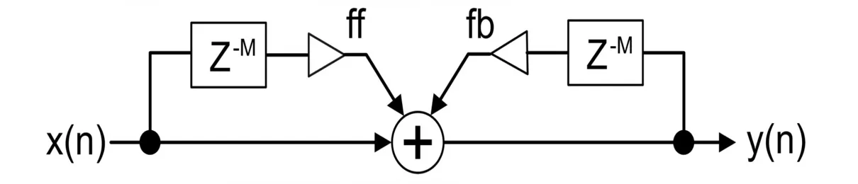
The Z blocks in the diagram use a superscript (Z-M) rather than Z-1 to represent that these blocks delay the signal by M samples rather than 1 sample, which means we’ll be using the delay operator rather than the history operator to translate this diagram.

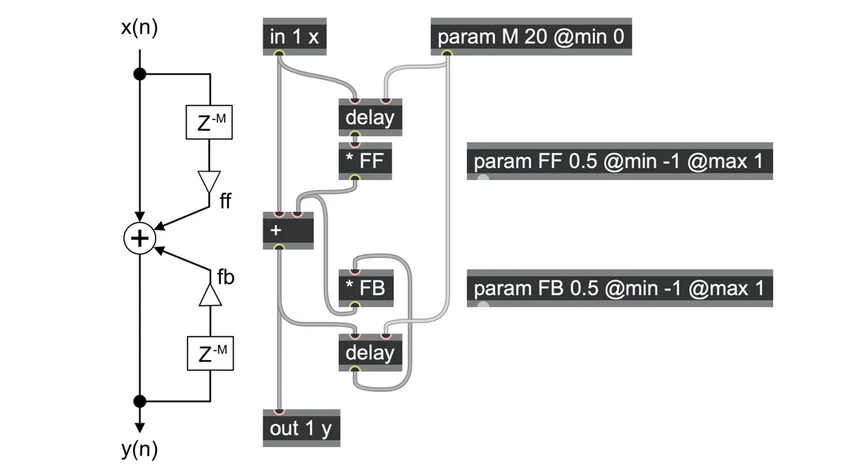
comb_filter.maxpat

If you use only the feedforward path (i.e., param FB = 0.0), it creates notches in the output spectrum.

If you use only the feedback path (param FF = 0.0), it creates peaks in the output spectrum of the sound.

Or you can combine both, creating both peaks and notches.

This should make it clear why it is called comb filtering: the spectrum looks a bit like a comb, with its peaks and/or troughs at evenly spaced frequencies. The specific frequencies where these occur depend on the delay length, with a peak at each whole number multiple of the delay’s fundamental frequency and a notch halfway between each peak. So, if your delay period is 10ms, corresponding to a fundamental frequency of 100Hz, there will be peaks at 0Hz, 100Hz, 200Hz, and so on, and notches at 50Hz, 150Hz, 250Hz, and so on.

However, if the param FF and param FB coefficients are negative, then this flips around, with notches at whole number multiples of the fundamental frequency and peaks halfway between. This is because any of the delayed frequencies that are in phase with each other sum together, while frequencies that are out of phase with each other cancel out.

Modulating the delay time produces a characteristic zooming sound as these peaks and notches slide up and down the spectrum together. It works especially well with spectrally rich harmonic sources such as pulse waves for the input.

Enharmonic combs

Our next filter block diagram is drawn from a paper authored by Jae hyun Ahn and Richard Dudas,[66] which begins with the goal of using delay-based filters to create “enharmonic” comb-like effects. That simply means that the delay periods of the two delays can be set at different frequencies that are not necessarily whole number harmonics, producing more complex spectra. Trial and error showed that they could create an elegant and great-sounding enharmonic filter that also remains stable using the following block diagram:[67]

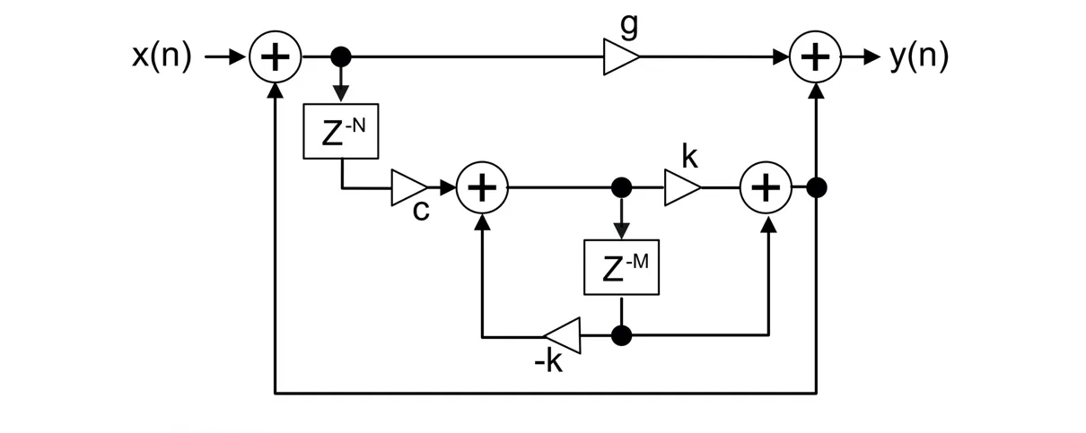
As before, we’ll rotate this block diagram and replace blocks with gen~ operator equivalents. As before, we replace param coefficients with inlets that will allow us to modulate our filter at audio rates, rearrange it for a more easily visible signal flow, and add some clipping for patch hygiene.

Here is the resulting patch, with the nested allpass filter highlighted in a box.

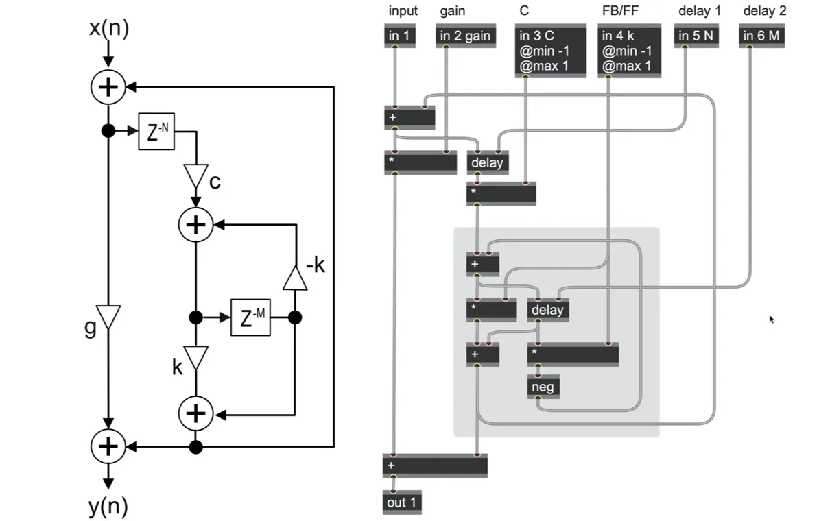
comb_enharmonic.maxpat

The comb_enharmonic.maxpat patch also shows an example of how to choose the two delay values using MIDI note semitones, which makes exploring the enharmonic output a lot of fun.

Strings

Delay times between 0.5 to 25ms and high levels of feedback can produce resonances evocative of string instruments. This method is commonly called Karplus–Strong string synthesis, after Kevin Karplus and Alexander Strong invented and analyzed it.[68] It is another kind of comb filtering but also a kind of dynamic wavetable synthesis in which the looping delay contents (the “tape”) represent one period of an oscillating sound.

This patch can work as a tuned resonator for any input sound, but if the input is just a very short burst of noise, it will sound like a simple plucked string.

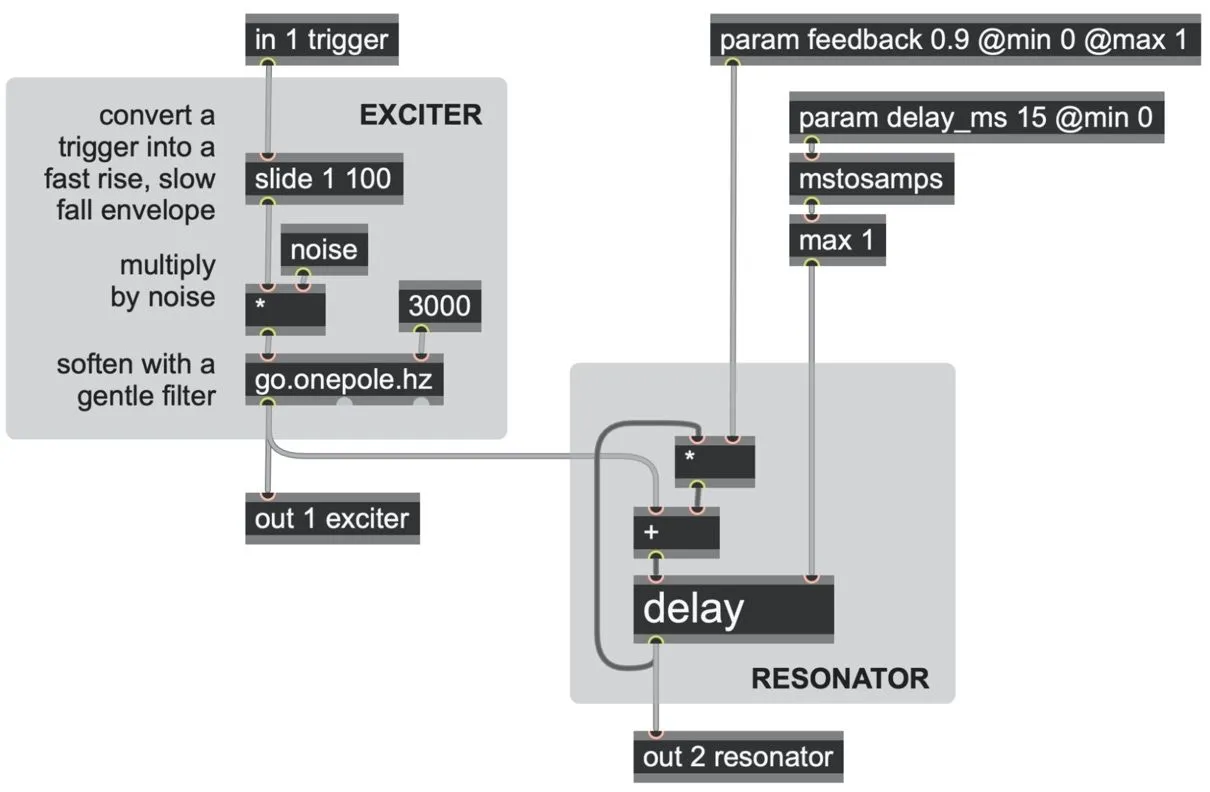
string_basic.maxpat

• The input noise is the exciter, which represents the input that sets the “instrument” in motion (like the interactions of the bow drawn across a string, a mallet striking a string or plate, or the interaction between a lip with a reed).

• The slowly decaying feedback delay acts as a resonator, which represents the physical system that the exciter acts upon. The pitch we set as the delay length is the lowest resonating frequency, but also any harmonic (any whole number multiple of the fundamental) can also resonate.

If we wanted to control this circuit with specific pitches, such as MIDI-style pitch numbers (in semitones), we would need a way to convert the pitch into an equivalent period in samples for the delay operator.

We can convert a MIDI-style pitch number into a frequency in Hertz using the mtof operator. A frequency in Hertz represents cycles per second, and so a reciprocal of this (using a !/ 1 reciprocal operator) gives us a period in seconds per cycle. We can convert this period in seconds to a period in samples by multiplying by the samplerate constant. We can even merge these two operations into a single !/ samplerate operator.

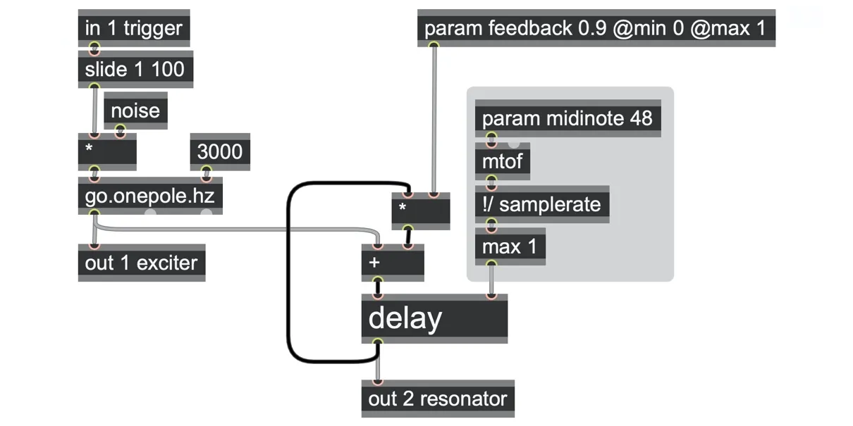
string_pitched.maxpat

The param feedback amount determines how long the string resonates (1.0 as infinite sustain, 0.9 or so for pizzicato), but this will vary according to the period of the delay. That Is, higher pitches with shorter delay periods will have shorter resonant decay times, and vice versa.

If this isn't desirable, we can use the same t60-based solution from delay_feedback_decaytime.maxpat to set a decay time in milliseconds independently of the string length. Now the strings will decay over the same amount of time (param decay_ms) regardless of whether they are high notes or low notes.

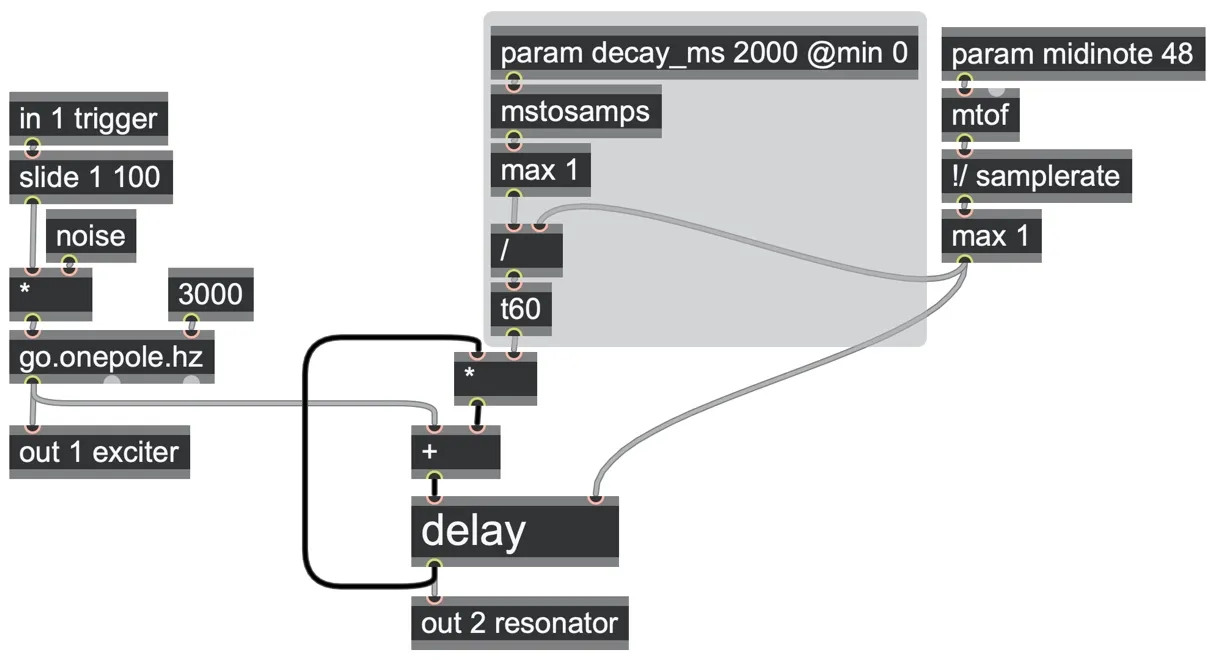
string_feedback_control.maxpat

What happens in the feedback loop?

We can refine this patch in several other ways, most of which involve placing more processing within the feedback loop.

1. With the feedback high and the delay time so short, it’s a good idea to add a highpass DC blocking filter into the loop, just as we did earlier in the chapter. This is also realistic: a physical string can’t accumulate DC endlessly, as the string is tied down to the body of the instrument, and the body dissipates this accumulated energy from the displacement of the string.

2. Changing the sign of the feedback also changes the sonic output: the alternation of positive and negative each time through the loop effectively makes the apparent period twice as long, sounding one octave lower (see the string_inverted_feedback.maxpat patch, for example). At the same time, this causes harmonic effects as the alternating positive and negative copies of the signal running through the loop largely cancel each other out. The result is a hollower tone of odd harmonics only, more characteristic of a wind instrument.

Spectrum of MIDI note C5 (about 532Hz), no inversion in the feedback loop.
Spectrum of MIDI note C5 (about 532Hz), inverting the signal in the feedback loop (apparent spectrum one octave lower).

Put another way, the resonant harmonic peaks of the spectrum of the inverted feedback case are exactly halfway between the resonant harmonic peaks of the non-inverted case. You might recall that we saw a similar phenomenon with positive and negative comb filter effects earlier in this chapter.

Damping

When you pluck a real string, the energy you impart to the system decays gradually, but the higher harmonics fade out sooner than the lower harmonics–the sound of the resonating string gets duller and duller after the initial pluck. We can emulate this easily enough by placing a lowpass filter into the delay loop, just as we did earlier in the chapter in the delay_feedback_filtered.maxpat patch.

However, the more subtle point is that using a lowpass filter will also impart some slight delay since, as we saw in Chapter 6, a low pass filter averages a signal with its own history.[69] Although it can be just a fraction of a sample, this delay is enough to cause the string’s pitch to drop slightly, and the string will sound “detuned” — the more filtering is applied, the more the string’s pitch drops.

We could compensate for this if we could estimate what the introduced delay will be and then shorten the core delay length by the same amount. The duration of additional delay a filter adds is dependent on the filter cutoff frequency and the particular filter algorithm we use. Unfortunately, the filter delay is also frequency-dependent — higher pitched tones may be delayed by slightly different proportions than lower-pitch tones (due to the filter’s complex phase response). The mathematics required to derive this is beyond the scope of this chapter, but for the case of the most basic one-pole filter with a mix coefficient (damping factor) of b, then 2*log(1-b) returns a close approximation to the required shortening of the delay time in samples. If we shorten the string length by this amount, we achieve a string simulation that can be damped without it going badly out of tune.[70]

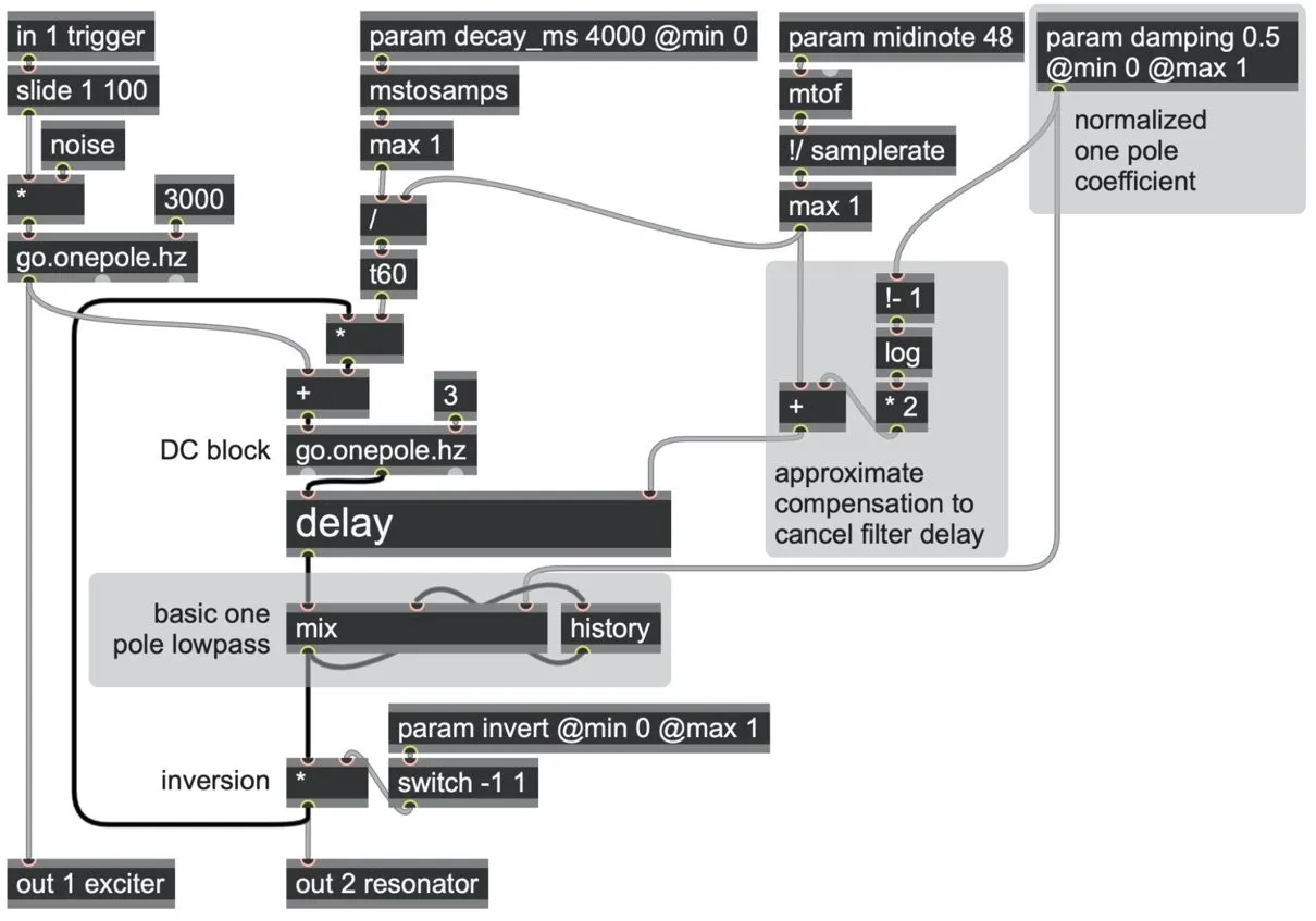
string_damping.maxpat

Cleaner interpolation for a consistent sound

Even if the damping filter is completely disabled (i.e., the param damping value is 0.0), you might notice that is sounds like there is still some damping happening, with the sound of the string after each pluck not just getting quieter but also becoming gradually duller as it fades away. You might also notice that this is stronger for some pitches than others. What’s going on?

In fact, this inherent damping is a side-effect of linear interpolation inside the delay operator itself. Why is there interpolation here? Briefly, any delay length that isn’t an exact whole number of samples requires some sort of interpolation to estimate the value between the sample frames of the delay's internal memory.

For example, if we wanted a delay time of exactly 7ms, we need a delay length of samplerate * 7/1000 samples, which for a typical samplerate of 44.1kHz works out to be 308.7 samples. But our delay’s internal memory tape is a discrete sequence of samples—there is no 308.7th sample! We could simply round this to the nearest whole number (by using delay @interp none), read the 309th value in the delay memory, and forget about the 0.7 part; but this will lead to distinct stepping or aliasing artifacts when our delay times are very short or gently modulated, such as in chorus and flanger effects, and especially for our string emulation here. Instead, we must estimate what the value of the signal would be at fractional points between samples, which means using some kind of interpolation.

The simplest estimation is to draw a straight line between samples and read off the value at the desired point in between. This is linear interpolation, and it is what the delay operator performs by default. Linear interpolation is computationally quite inexpensive and very effective for most delay purposes. However, as we saw in the last chapter, there is a close relationship between linear interpolation and low pass filtering; and with the very short delay times and high levels of feedback in string emulation, this low pass filtering effect becomes noticeable. To solve this problem, we need a form of interpolation that does not change the frequency spectrum. [71] Let’s look at a couple of solutions.

In Chapter 6, we looked at a kind of filter that has no effect on the frequency spectrum: the allpass filter. This is typically described as a filter that applies a change of phase, but another way of looking at it is that it applies fractional sample delays. Theoretically, the allpass filter we looked at (go.allpass) can apply a delay between 0 and 2 samples’ duration. If the desired delay is D samples, then the allpass coefficient can be calculated as (D-1)/(D+1). So we could solve our problem by combining a regular, non-interpolating delay @interp none operator for the integer part and a go.allpass filter for the fractional part, which together should let us have any delay time we want.

There’s just a slight wrinkle: the allpass filter’s response becomes distorted at the extremes of its range and is better behaved between a range of about 0.3 and 1.3 samples’ delay, so it’s best if we can keep our use of the allpass filter within that range. We can ensure that by sending our desired delay time through a wrap 0.3 1.3 operator for the allpass filter, and we can subtract that from our desired delay to get a remainder (that will always be a whole number) for the delay @interp none part. This works brilliantly, providing clean, unfiltered delays even at non-integer lengths.

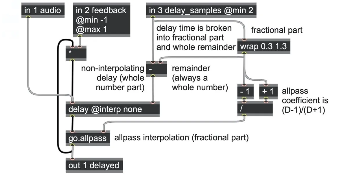
delay-interpolation-types.maxpat

Unfortunately, there’s one more catch: if we want to modulate our delay time continuously, say with an LFO, we will find that in some circumstances, the allpass filter starts to resonate and become harsh or even explodes (watch your ears!). For example, this can happen if the LFO period is a simple whole number division of the delay time, such as one-half. If we’re trying to emulate a physical string, this might not be a problem. Any physical modulation (such as from a whammy bar on an electric guitar) would be at a much lower frequency than the string itself. But for more exploratory synthesis, including audible frequency modulation of a string, we would need to handle this case.

The cheapest solution would be to add a saturator in the feedback loop, just as we did earlier in the chapter. You can see an example of this in the string_everything.maxpat patch.

Alternatively, we could try to tackle the cause of the problem, which is the feedback loops inside the allpass filter itself. Like almost all the filters we explored in Chapter 6, the allpass is an example of an Infinite Impulse Response (IIR) filter. It is infinite because it contains a feedback loop that operates on the histories of its own outputs. A different class of filters, Finite Impulse Response (FIR) filters, do not contain feedback and only operate on the histories of their inputs. That is, they only have feedforward paths.[72] FIR filters are often more expensive or require more data to achieve comparable results to IIR filters, but their avoidance of feedback paths means they are far more stable under modulation. This also makes them valuable for interpolation and resampling applications.

For the purposes of our delay interpolation problem, we can use an FIR filter that performs sinc interpolation. We’ll look at what sinc interpolation is and why it works in more detail in Chapter 9, but briefly stated, the sinc function sin(x)/x happens to be an ideal smoothing curve for resampling without losing high frequency energy up to a certain point. In our patch below, we use an 8-point sinc interpolation, which means we read out eight non-interpolated samples from the delay operator, each spaced one sample apart, and multiply each one with an evenly spaced slice of a windowed-sinc function, shifted by the fractional part of the delay time, adding them all up for our output value.

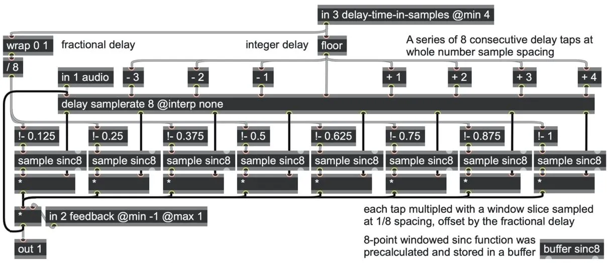
delay-interpolation-types.maxpat

This solution is more expensive than an allpass filter, but it does a very good job of preserving the spectrum up to samplerate/4. It is also far more robust under more extreme modulation as long as the modulation frequency is not higher than the fundamental frequency of the string itself. This may be a preferable solution if you want to explore very deep phase modulation, as we will see in the next chapter.

We will return to look at more refined physical models in Book 2.