Appearance
Chapter 10:
Windows of Time
In this chapter, we’ll be looking at how we can reset timelines and lifespans: using one process to determine the durations of another process repeatedly. What do we mean by timelines and lifespans? We’ve already seen examples of nesting timelines by subdividing and synchronizing ramps in Chapter 2. For example, even a simple repeating drum hit has at least three nested spans of time: the periodic tempo, the duration of the drum sound, and the period of the waveform that makes this sound.
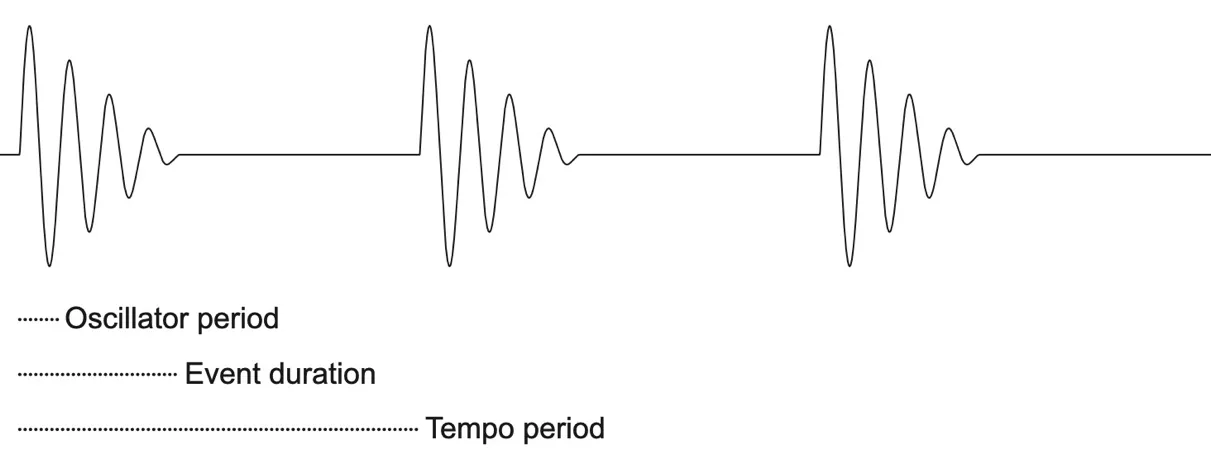
Note that two of these layers are periodic (the potentially endlessly repeating layers of the oscillator and the tempo), while the layer between represents a finite “window” of time (the lifespan of each event). In this chapter, we’re going to dig deeper into these kinds of nested cyclic and windowed durations, right down to microsonic scales of pitches and timbre, producing a variety of formant, pulsar, polyphonic granular, and hard sync synthesis results.
Sync
Hard sync is one of the simplest examples of one process defining the lifespan of another—by literally cutting it short. Oscillator hard sync is a classic technique in analog synthesis in which one oscillator’s phase (let’s call it the “carrier”) is reset back to the start whenever another oscillator (let’s call it the “scheduler”) completes a cycle.
A hard sync reset causes a jump in the phase of the carrier (so, in a way, this is also a special case of phase modulation). The reset jump will likely cut the carrier’s waveform partway through one of its cycles.
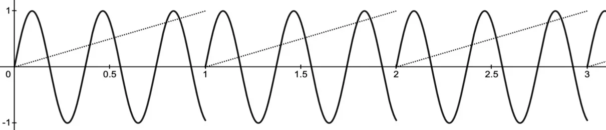
The graph shows a sinusoidal carrier oscillator at 2.7Hz (solid line) being hard synced by a scheduler phasor oscillator running at 1Hz (dotted line), producing a hard cut in the carrier waveform once per second. When listening to the carrier, hard sync produces a complex of the two oscillator tones. However, typically the scheduler’s frequency is what we hear as the main pitch, while the carrier frequency shapes the principal formant or harmonic tone. Holding the scheduler’s frequency constant while sweeping the frequency of the carrier creates a tearing or zippering sound—that’s what people usually think of as the characteristic sound of hard sync.
A tentative hard sync patch in gen~ might look something like the following patch:
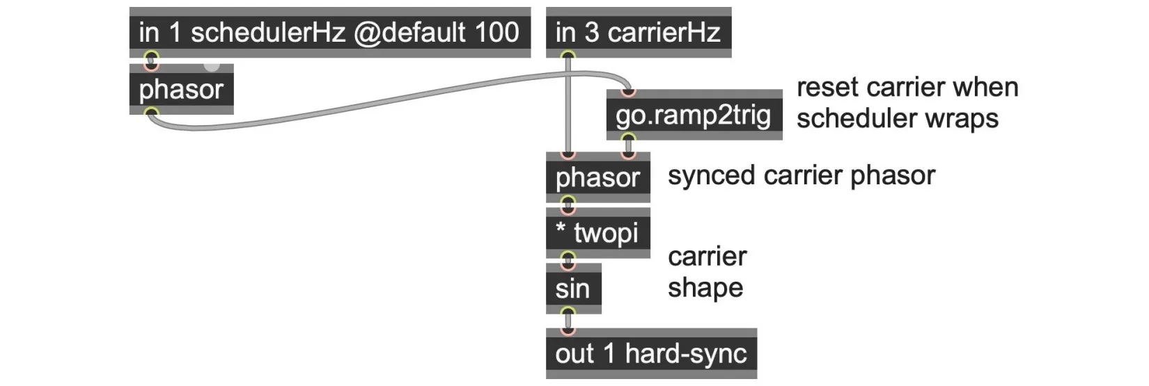
Here, we derive triggers from the scheduler phasor using a go.ramp2trig abstraction and use those triggers to reset the carrier phasor back to zero using the phasor operator’s right inlet. This does work, but it will likely suffer from aliasing noise. Even if the carrier is a smooth sinusoid, the periodic hard sync cuts in the waveform will produce a lot of high-frequency harmonics in the same way that the large jumps in sawtooth and square/pulse-shaped waveforms do. The strength of these harmonics produces the desired brightness of a saw/pulse or hard sync sound. They are also problematic for digital synthesis. as they can very easily lead to harsh aliasing noise. At the end of this chapter, we will return to develop an understanding of this noise and build a solution to suppress it, but first, we will look at a much simpler related synthesis technique known as windowed sync.
Windowed Sync
Windowed sync is a variant of oscillator sync popularized by digital phase distortion synthesizers. It eliminates most of the aliasing problems of a hard sync cut point by simply fading out the carrier waveform right at the moment the sync cut happens. Perhaps this might seem like cheating, but it’s quite pragmatic, cheap, and effective.
All you need to do is amplitude modulate the carrier using some kind of envelope or window function that fades down to 0.0 right at the cut point.
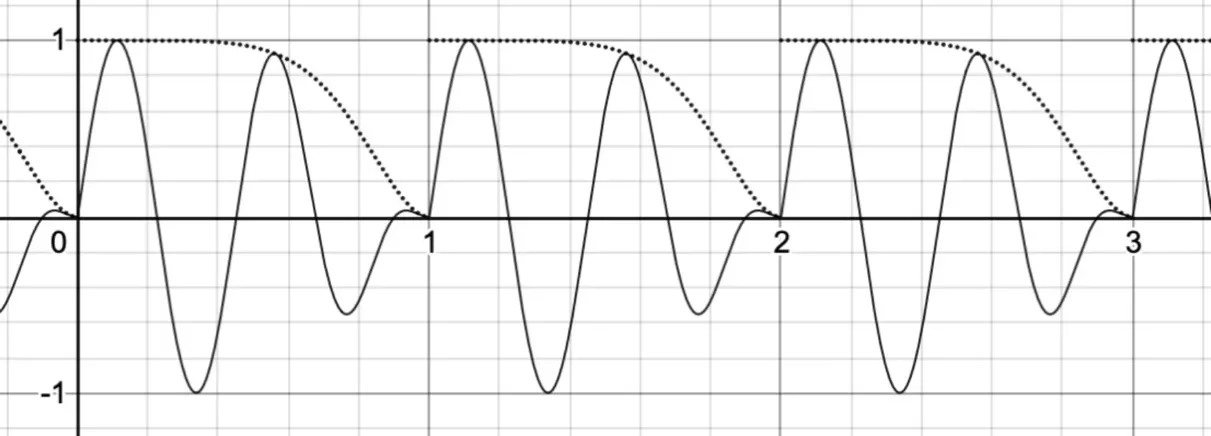
In the graph above, a smooth window function (dotted line) derived from the scheduler phasor is used to amplitude-modulate the synced carrier waveform such that the amplitude falls to zero at the sync point (solid line).
Here is what that might look like as a patch.
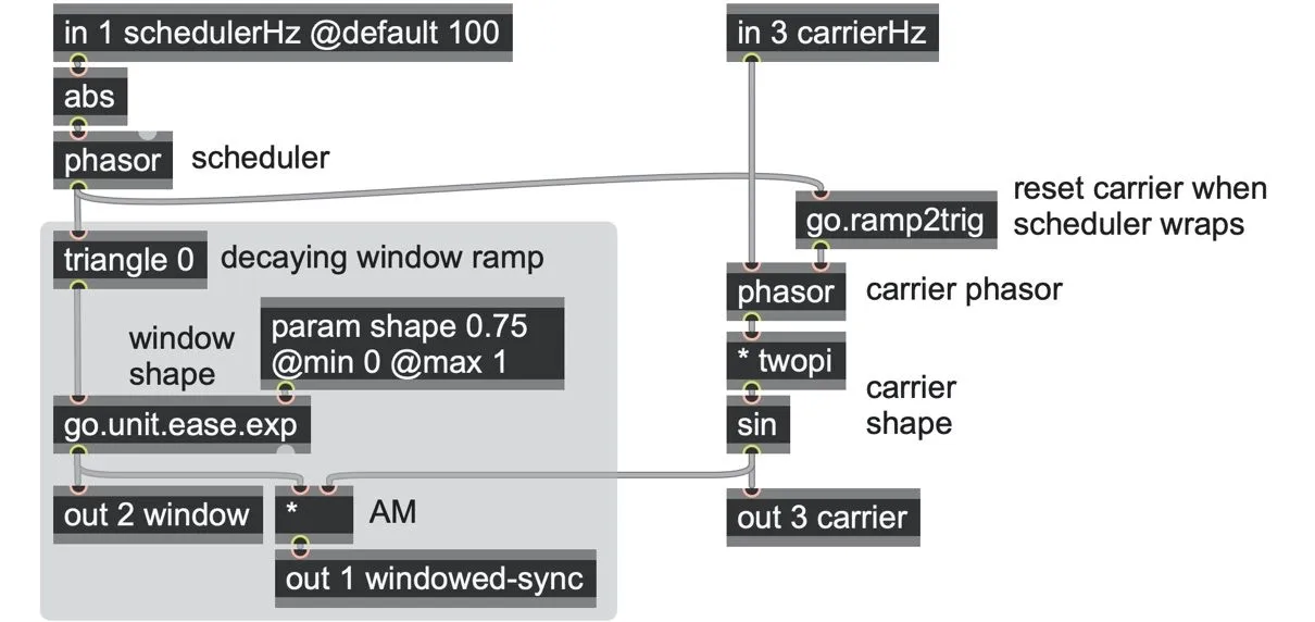
To create the window, we invert the unipolar scheduler’s phasor so that it runs from 1.0 down to 0.0 as a linear decay shape (using a triangle 0 operator) and then apply a go.unit.ease.exp abstraction to produce a curved envelope shape similar to the graph above. You can try substituting this shape with other options from the unit shapers in Chapter 3. This window output is then multiplied with the carrier waveform and output at out 1.
If you compare the windowed sync sound of out 1 with the raw hard sync signal at out 3, you will be able to hear how windowing has suppressed a lot of the harsh aliasing, without losing too much energy at the lower harmonics. Here are the two spectra compared (windowed sync in black, raw hard sync in gray):
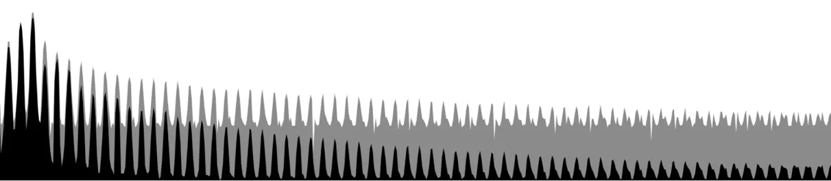
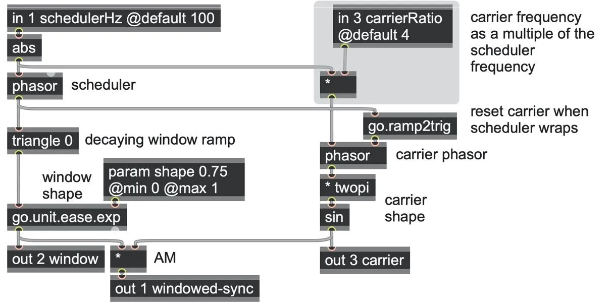
Sweeping the carrier frequency above the scheduler frequency now sounds a bit like a filter, where the carrier frequency picks out which harmonic resonates the most. In fact, it picks the next harmonic in the series for each multiple of the scheduler frequency. For example, if the scheduler frequency is 200Hz, the harmonics are picked out one by one when the carrier is 200Hz, 400Hz, 600Hz, and so on. So, rather than specifying the carrier frequency independently of the scheduler frequency, perhaps we should take inspiration from what we learned in Chapter 8 and work with a carrier-to-scheduler ratio. In this case, we may prefer to set the carrier as a formant multiplier of the scheduler frequency.
Sub-sample accuracy
There’s one more important refinement to make. If you listen carefully at higher scheduler frequencies, you might still hear some aliasing noise. The source of this noise is still the carrier phasor reset, but the reason is a bit more subtle. Specifically, we shouldn’t be resetting the phase of the carrier exactly to zero but to some value near-zero that properly reflects the ideal phase at that point. That’s because the ideal reset probably happens somewhere between one sample frame and the next. If we zoom right down to the sample level, we can see that an ideal scheduler phasor (dotted line in the following graph) wraps somewhere between actual sample frames. Within the sample frame in which the phasor wraps (marked in gray), the sample value is slightly above zero.
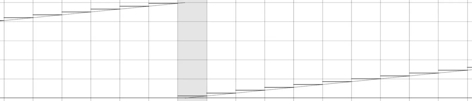
In contrast, when a phasor operator is reset by a trigger to its right inlet, it always resets to zero exactly. Although the difference looks small, it can have quite a significant effect on the sonic quality of the output (and we’ll be seeing the importance of subsample offsets like these again and again throughout this chapter).
To fix this in our patch, we’ll have to replace our carrier’s phasor operator with an equivalent accumulator, using the same history, +, and switch operator set we’ve seen since Chapter 2. That way, we can control what value it resets to. This accumulator counts using a slope that is relative to the scheduler’s slope (which could be derived via go.ramp2slope abstraction or simply by schedulerHz/samplerate). And as the crucial step for subsample accuracy, the accumulator’s switch operator doesn’t reset to zero but to a phase that is relative to the scheduler’s phase whenever the scheduler itself wraps.
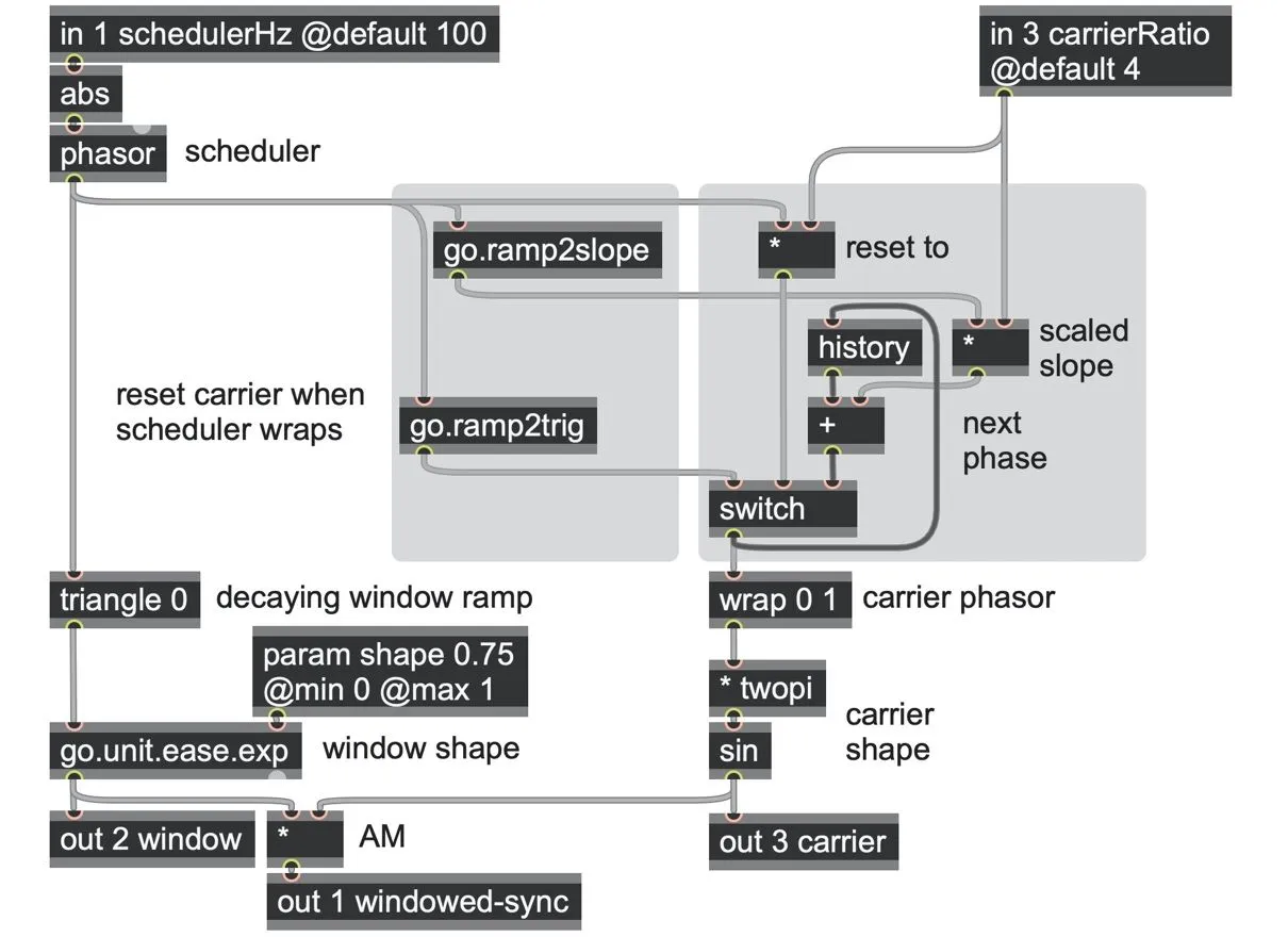
windowed-sync.maxpat
And with that, we have a very effective windowed-sync patch. With the scheduler at a low frequency, e.g., 100Hz, and the carrier exponentially ramping down from a high to lower frequency (e.g., 2000Hz to 100Hz), it can be a little reminiscent of a classic Roland 303 acid sound.
One of the neatest things about this method is its generality. Practically any envelope shape can be substituted here, and any carrier waveform, so long as either the start of the carrier waveform or the start of the envelope waveform begins at zero, and the envelope ends at zero. You could try swapping out the sine carrier shape with a wavetable oscillator from Chapter 9, for example, or an FM oscillator from Chapter 8.
In fact, we already saw a somewhat similar patch to this toward the end of Chapter 8. The last Modified FM example also performed an amplitude modulation of a carrier waveform with a window function (in that example, a raised cosine shape), leading to a sound with strong formant qualities. In that example, the more the window shape is squeezed, the more silence appears between the blips, and the more the formant is expressed.
Pulsar Synthesis
As we saw back in Chapter 2, we can take a phasor ramp and multiply it by some number greater than one to get a ramp whose slope is steeper. If we then use a clip 0 1 operation to limit this steeper ramp into the 0.0 to 1.0 range, we get a shorter ramp that nevertheless still recurs at the original rate.

Dotted line: A scheduler phasor at 1Hz.
Solid line: The same phasor multiplied by 5 and clipped between 0 and 1.
We can apply this idea to our windowed sync patch in order to insert silence between grains, simply by scaling and clipping the scheduler phasor before it is shaped into a window, and using a param windowRatio to set the scaling factor.
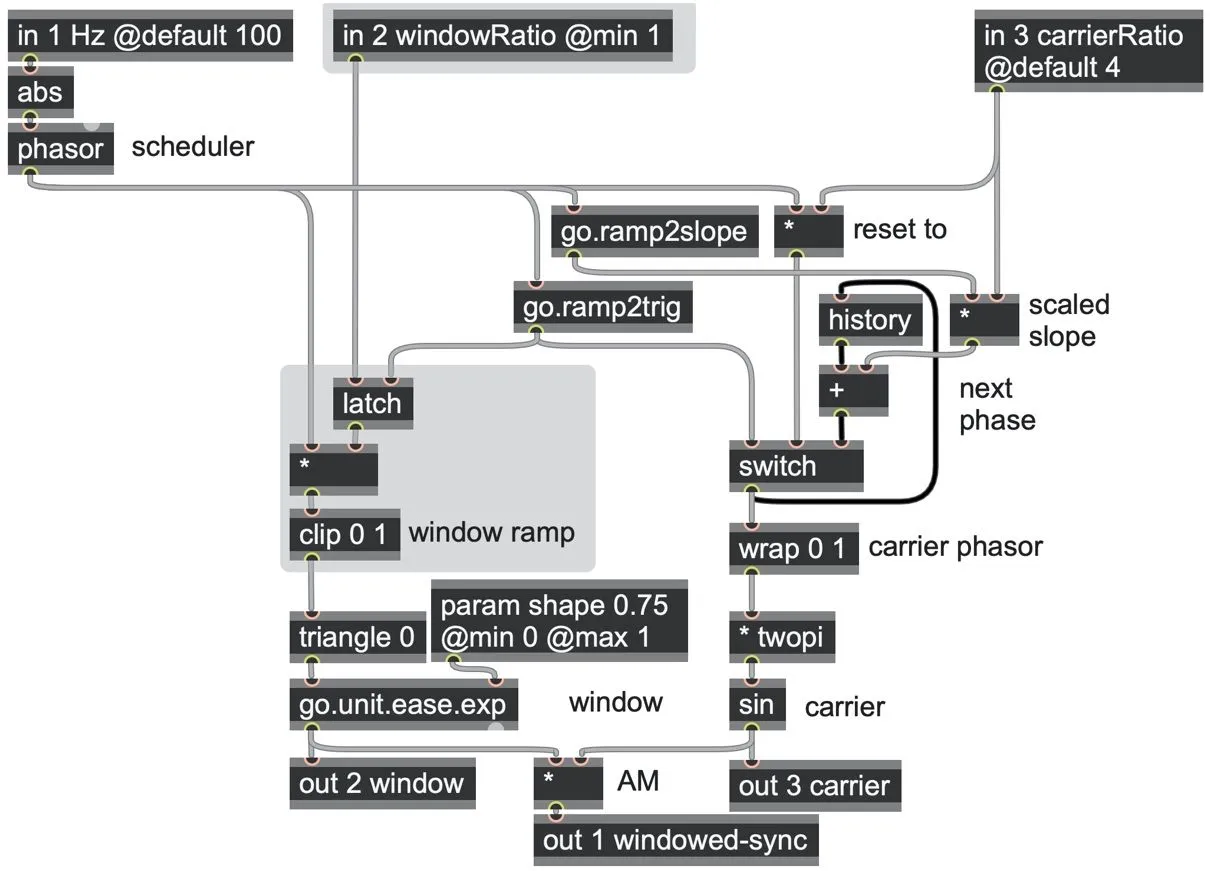
pulsar.maxpat
It’s quite remarkable how much this patch can sound like a resonant filter, with the carrier ratio determining the resonant peak and the window ratio (and shape) of the resonance, even though there is no filter involved, and all we are actually doing is inserting silence!
What we have created here is also a form of synchronous granular synthesis known as pulsar synthesis.[101] Granular synthesis encompasses a variety of techniques that mostly involve scheduling many tiny particles of sound rather like clouds of tiny notes with durations in ranges of milliseconds. Each grain is typically a combination of two components: a carrier signal (which could be synthesized, read from a buffer, read from a delay, etc.) and an envelope to define the overall amplitude shape. That is, much like the diagram at the start of this chapter, granular methods usually incorporate three layers of schedulers, envelopes, and carriers. We’ll be exploring several granular examples in this chapter and more granular techniques in Book 2.
Pulsar synthesis is a specific kind of granular synthesis that uses synchronous scheduling, meaning that grains are scheduled at a periodic rate that imparts a fundamental frequency to the sound. Within this period, there is a grain called a pulsaret, followed by a period of silence. That is, the duration of the sounding pulsaret is typically briefer than the period of the scheduler. The ratio of these two durations creates the effect of a duty cycle[102], and modulation of it creates an effect related to pulse-width modulation. If the carrier is pitched, it will likely have a higher frequency than the scheduler, and this can convey a formant frequency.. The way the length of the window duty cycle shapes the spectrum is easy to understand. With a longer window, more cycles of the underlying carrier waveform can be heard, and thus the more the carrier frequency dominates the sound (which is what evokes the character of a resonant formant filter). Conversely, as the window becomes shorter, fewer cycles of the carrier can be heard, until the waveform becomes more of a blip whose wide-band spectrum depends more on the window shape itself.[103]
Pulsar synthesis is quite a general technique: the carrier can be an arbitrary finite sound, and any window shape can be used for the envelope. For example, in the following patch, we modified our pulsar.maxpat patch to use a variable Tukey window shape and added another harmonic oscillator routed to act as an FM modulator of the carrier for a much more complex sonic output. It’s well worth exploring extensive frequency modulation of the inputs of this patch.
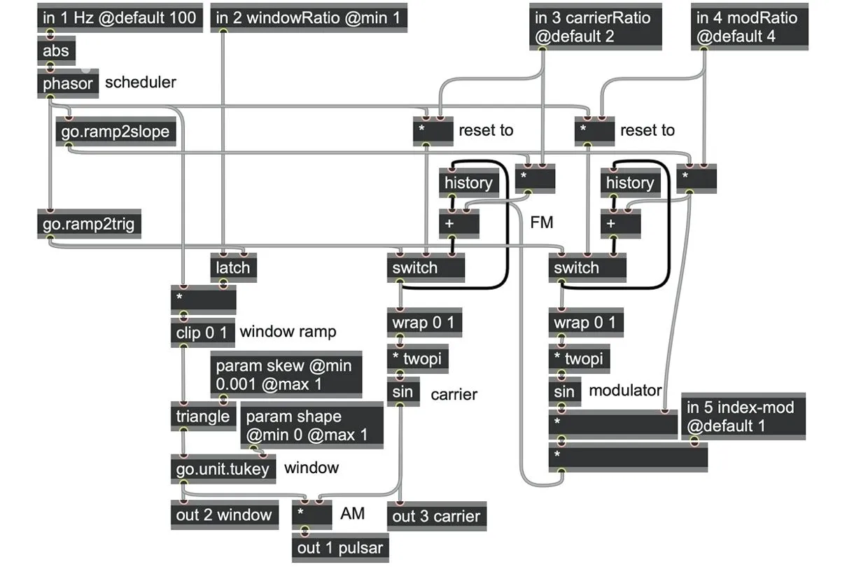
pulsar_fm.maxpat
When the event duration is longer than the fundamental period
Why is param windowRatio limited to @min 1? A ratio less than one would imply a duty cycle greater than one, which means that the envelope duration becomes longer than the available time in the scheduler period. With the patches we have built so far, this would simply mean that the envelope would never reach the end before a new envelope begins, truncating the waveform mid-cycle and losing the benefits of the windowing.
There are a couple of alternate strategies we could try here. First, we could prevent any new envelope from starting until the current envelope has actually completed, which will create a kind of subharmonic effect. Alternatively, we could modify our algorithm to support multiple overlapping grains at once as a kind of polyphony. We’ll look at both of these solutions in the next sections.
Suppressing retriggers (subharmonics)
The first way to allow grain windows that are longer than the scheduler period is simply to prevent the scheduler from starting a new window until the last window has been completed. (This is similar to the behavior of envelope generators that will not retrigger until the current envelope completes). To do this, we will first need to decouple the window ramp generation from the scheduler ramp in just the same way as we already did for the carrier.
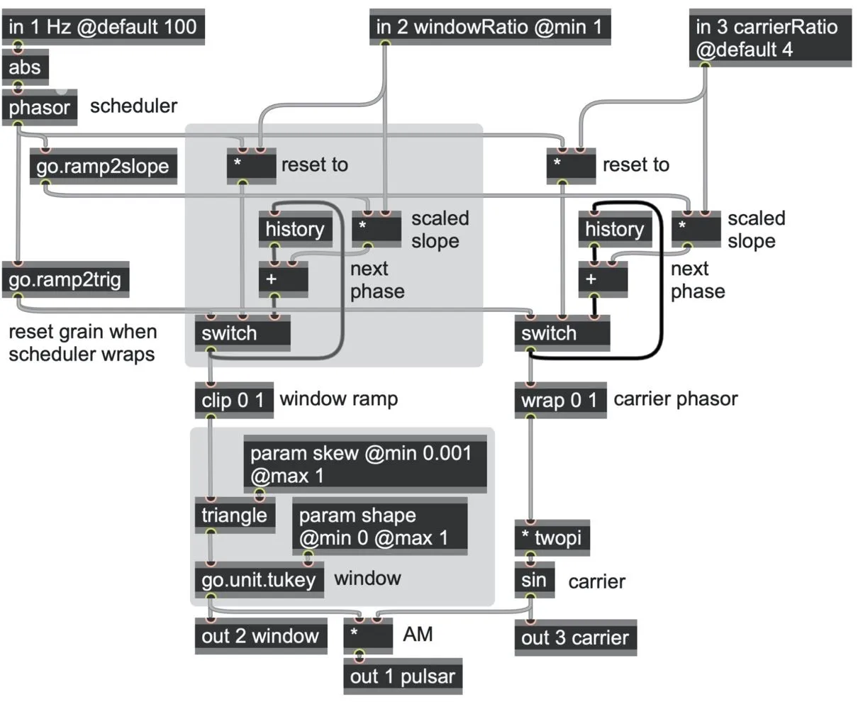
Now that the window ramp runs independently of the scheduler, we can suppress a new grain from being started by bypassing (zeroing) the scheduler’s go.ramp2trig triggers. Our goal is to suppress these triggers only while our window is busy ramping. We know our window envelope is still busy if the window ramp phase has not reached 1.0 yet, which means we can test the ramp phase using a < 1 comparator.
We can use this logical condition to suppress the scheduler’s go.ramp2trig triggers with an and and a not operator. In other words, our grain envelope (and carrier) ramps will only be reset if the scheduler triggers and we are not already busy.
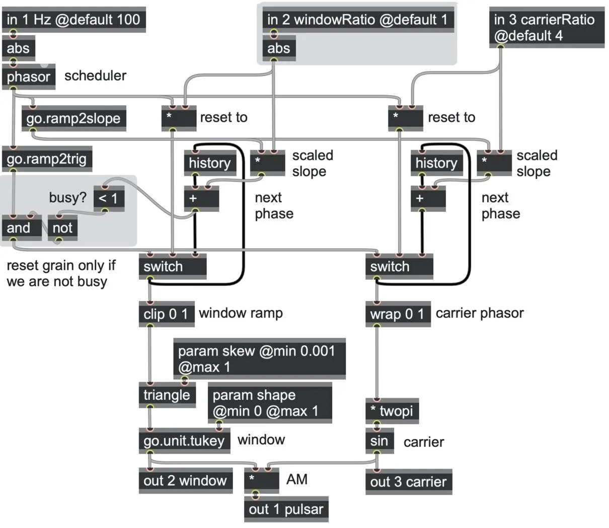
pulsar_subharmonic.maxpat
Now, while param windowRatio is greater than 1.0, this patch behaves as it did before, but if you bring the param windowRatio below 1.0 toward zero, you will hear the frequency halve, then divide into thirds, quarters, and so on, picking out the subharmonic series of the fundamental scheduler frequency. If the scheduler frequency is fairly low, say around 100Hz, then these subharmonics will quickly enter the temporal space of rhythms.
To hear the subharmonics as pitched tones, try setting the scheduler frequency high, say around 1000Hz, and then slowly bring the param windowRatio down from 1.0 to 0.5, then 0.3, then 0.2, etc. The envelope generator is no longer completely subordinate to the scheduler phasor but can also ignore it when it is already busy.
Polyphony (distributing event triggers)
What if, instead of truncating or suppressing long event windows, we wanted them all to play out fully, overlapping on top of each other like the notes of a polyphonic instrument? In this section, we’ll look at one method to do this and another one later in the chapter. We’ll first describe things in terms of note-playing because it makes an easier analogy, but we will then translate it to the grains of granular synthesis.
Strictly speaking, the operators of a gen~ patch, like all serial computing systems, can only process one thing at a time. So, just as we need at least three fingers to play a three-note chord on a keyboard or three singers to sing three-part harmony, we can imagine that we would need a separate signal process, or “voice,” for each potential overlapping note for a polyphonic patch. One of the simplest ways to achieve this is to make a copy of a subpatch for each voice. Then, if we have some kind of scheduler producing triggers for note events, then all we need is an algorithm that will distribute each new trigger to one of the voices.
The simplest distribution algorithm just sends each new event to the next voice in turn (sometimes called the “round-robin” method), which could be done with a counter and gate operator like this:
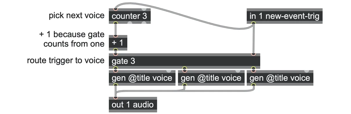
However, this algorithm isn’t very practical if some notes are short while others are long: a long-held note may be cut off too soon as its voice is reused for another note, even if there were other voices not busy playing anything. It would be better if we could delegate this responsibility to the voices themselves so that a voice could say the equivalent of “Sorry, I’m busy, let me ask the next person.” Then, we can pass each new event trigger to the first voice, and if this voice was already busy playing a note, it would pass the event trigger on to the next voice, and so on, until the new event trigger reaches a voice that isn’t already busy and can start the new note.
We already saw with the subharmonic pulsar synthesis example how we can use the envelope to determine whether a patch is busy playing an event and to ignore new triggers if it is. We can use essentially the same logic control here, simply using a gate operator to determine whether to handle a new event trigger within the voice subpatch (if the voice isn’t busy) or route the trigger to an outlet for the next the voice subpatch (if the voice is busy). A simple example might look like the following:
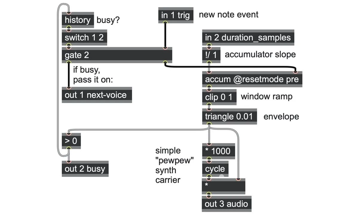
gen @title voice
The core of the patch is the accum and clip 0 1 operator pair that ramps from 0.0 to 1.0 over the duration of an event. The slope of the ramp is set from the duration in samples via a !/ 1 operator, and the ramp is shaped into a fast attack, slow decay envelope here using a triangle 0.01 operator. As long as this envelope’s output is greater than zero (via the > 0 operator), we know the voice is currently busy.
This “busy” state is fed back via a history operator to control the routing of a gate operator, to either handle the input trigger inside the patch (by restarting the accumulator) or, if busy, to pass it on to the out 1 for the next voice. We highlighted the trigger signals with black patch cords to make this structure clearer. (The bottom part of this patch just derives an enveloped sine sweep from the window ramp itself—it’s not important to the polyphonic method here, it’s just something simple so that we can hear that it is working.)
We can now duplicate this voice subpatch several times and chain them together.
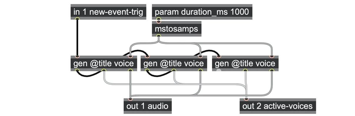
Notice how the parameters are sent to all voices, and all the voices’ audio outputs are added together at out 1. Summing up the “busy” states of each voice subpatch (from their 2nd outlets to out 2) also tells us how many voices are active at any time. The trigger signals (again here marked with black patch cords) are routed from one voice to the next as they pass along any trigger they can’t handle themselves.
You could trigger the events from a MIDI input source, any of the random trigger generators we saw in Chapter 4, or sequencers from Chapter 5. This patch can now play up to three overlapping sounds at any time without cutting any off midway. To increase the maximum polyphony, just add more voice subpatches!
Polyphonic notes
The voice subpatch can be practically any synthesis algorithm; all it needs is some way to indicate whether it is busy or not and the trigger handling/forwarding subcircuit. However, the more voices we add, and the more controls we add to each subpatch, the more spaghetti-like our patching can become.
Here is a little trick to simplify things: if we store the shared controls into named history operators in the parent gen~ patch, then these names will be available to reference in subpatches (and the same holds for param, buffer, and data operators).
For example, in the following patch, we store both the required slope and frequency as history slope and history freq, respectively, for a requested note duration and pitch.
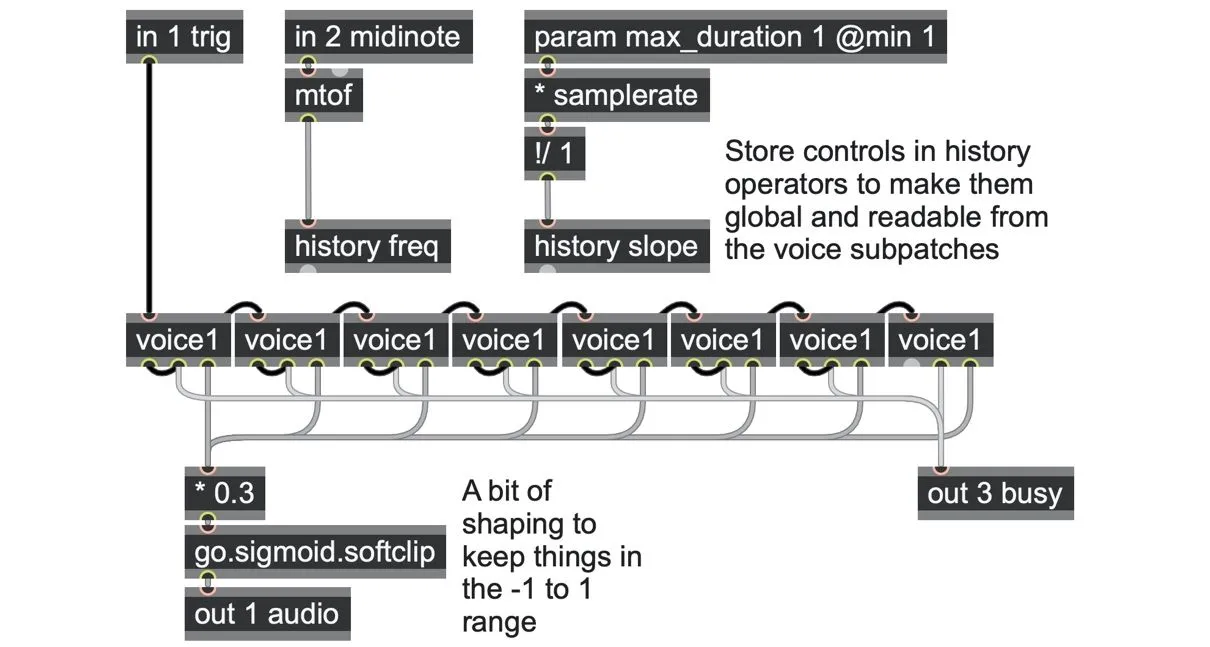
poly_voices.maxpat
We also increased the number of voices, and we saved the voice subpatch as an abstraction on disk next to the main patch (with the name voice1.gendsp) so that we only ever have to modify one subpatch, and all the others will update accordingly. We also scaled down the output and applied a wave shaping soft limiter to the combined audio output. When many notes overlap, it’s quite possible for the total signal amplitude to go outside the -1.0 to +1.0 range, so a bit of attenuation and limiting may be a good idea for any kind of polyphonic patch.
Here’s the voice1 subpatch, making reference to the history slope and history freq values by name (and adding a bit of random deviation for interest):
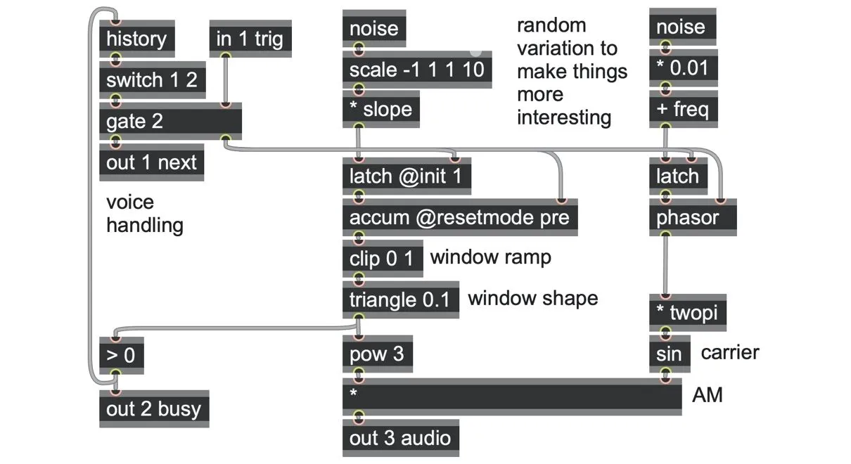
voice1.gendsp
Granulation
To bring things back toward the microsonic realm of granular synthesis, let’s build a voice that plays microsonic snatches from a wave file stored in a buffer src operator. A starting patch might look something like this:
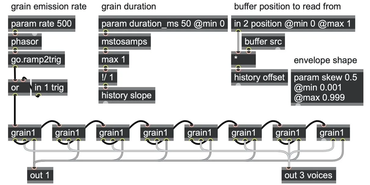
poly_granulation1.maxpat
The trigger source is a phasor fed into a go.ramp2trig, but there’s also the option of external triggering via the in 1 operator, combined via the or operator to let either trigger source pass through. The grain parameters include:
a grain duration that is converted from milliseconds to a per-sample ramp slope and made global via the history slope operator
a relative position from the audio buffer (via in 2), which is converted to a sample index and made global via the history offset operator
a global envelope shaping option via the param skew operator
All of these global names (“slope,” “offset,” and “skew”) are referenced inside the grain1.gendsp abstraction, which looks like this:
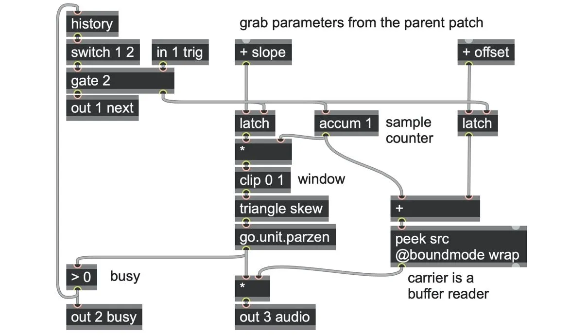
grain1.gendsp
The voice handling here is unchanged. The core is now a sample counter (the accum 1 operator) that is reset to zero whenever a new grain starts, adding one for every passing sample frame. This is multiplied by the slope, as captured at the start of the grain via a latch operator, and clipped into 0.0 to 1.0 to create the envelope ramp. The envelope is shaped by a triangle that references the global skew parameter, and we shaped it using the go.unit.parzen window unit shaper. The sample accumulator is also used to read from the buffer src, shifted by the global “offset” parameter (also latched to hold it constant throughout the grain), and fed into a peek src operator with @boundmode wrap to ensure reading off the end of the buffer will wrap around to the beginning.
Asynchronous and stochastic grains
Patches like these respond really well to the introduction of randomized deviations to their parameters. Iannis Xenakis, the pioneering composer of microsound, argued strongly for the introduction of stochastic and probabilistic organizations of individual grains to re-introduce the micro-fluctuations and variance of timbre that make real acoustics sound more alive than electronic sounds made of pure harmonics.[104]
For example, even very slight deviations (on the order of 0.1%) in the buffer offset, so that each grain is reading from a slightly different part of the buffer, can completely transform the sonic character of the result. Meanwhile, deviating the emission rate very quickly eliminates any sense of pitch from the scheduler, which instead turns into a kind of probabilistic density. Note that emission rate and emission density are both concepts of frequency, but one is regular (and pitched), and the other one is irregular (and unpitched).
Here are both of these variations in the poly_granulation2.maxpat example:
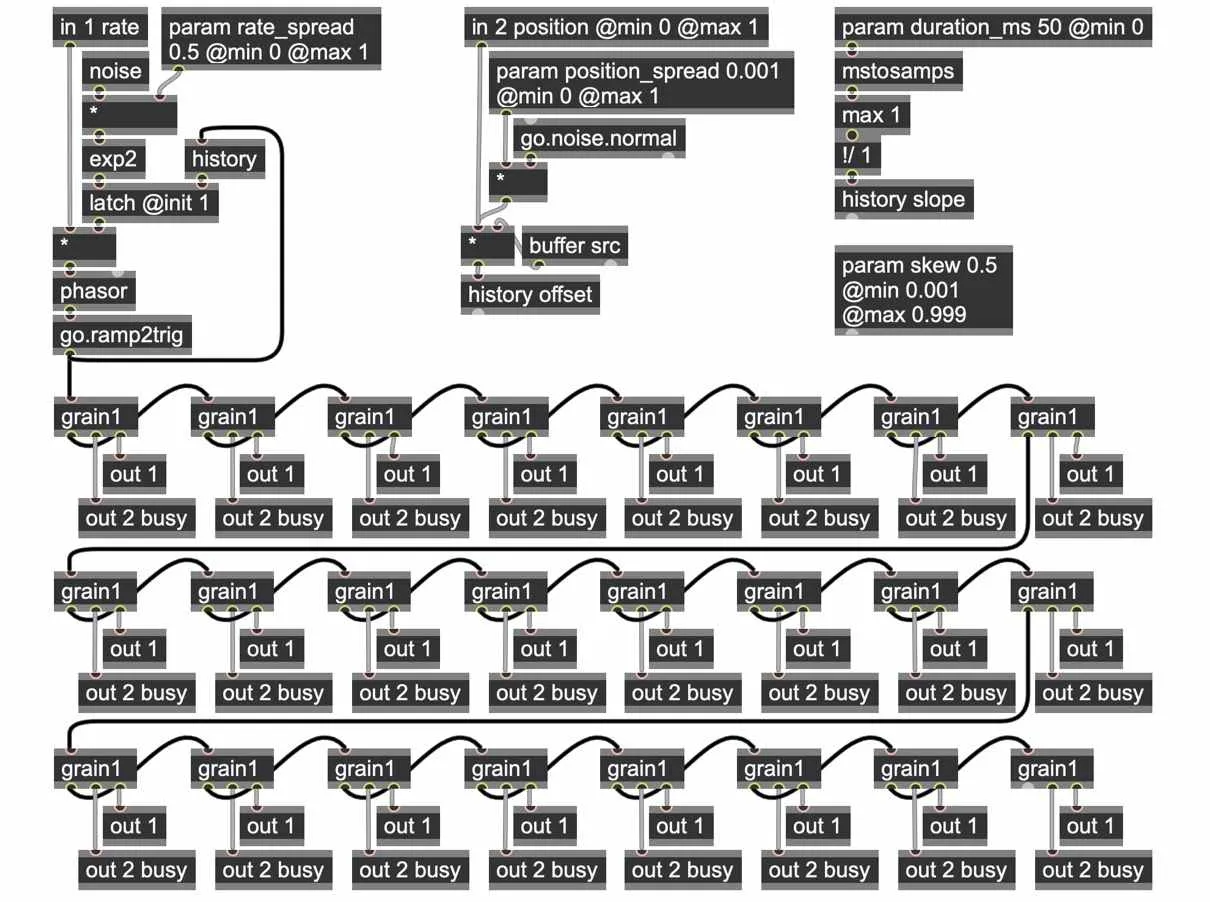
With a low emission frequency of around 1-10Hz, durations of around 100-200ms, and a fast attack skew of 0.1 or less, this will create clear percussive events. Softening the skew to an even 0.5 and increasing the emission frequency to around 100Hz or higher will start to create a dense, cloud-like sound. Bringing the duration down to below around 20ms, the original content of the buffer will seem to fragment into tiny particles of sound.
There are lots more refinements we can add to this, including adding randomized amplitude per grain, randomized stereo pan and width, variable playback speed per grain with deviations, and so on. For the most part, this is just an extrapolation of the techniques we’ve already explored, and several of these ideas are demonstrated in the poly_granulation3.maxpat example. You could also try embedding some of the wavetable or wave terrain ideas from Chapter 9 into the grain patch to give each grain a unique trajectory through data space!
But there’s one more detail we’d like to address. If you turn all the stochastic parameters to zero, set the grain size to just a couple of milliseconds, and set the emission rate to an audible pitched frequency, you might notice the noise of aliasing recurring again. We’ll look at that next.
Subsample-accurate events from phasor ramps
The polyphonic patches we have created so far trigger grains with sample-accurate timing, in the sense that the trigger aligns each grain to the precise sample frame during which the phasor ramp wraps. This is already much more precise than typical “control rates” and MIDI timing. But the smaller the grains get, and the faster they are spawned, the more the sound can transform into a pitched oscillator; and as we saw with windowed sync (and pulsar synthesis) earlier this chapter, at these rates, being sample-accurate just isn’t accurate enough. At these rates, the fractional subsample locations of events become very important, and we need to locate each event precisely within a sample frame with sub-sample accuracy.
Let’s zoom right in to where the scheduler phasor wraps and take a look at the grain envelope it causes:
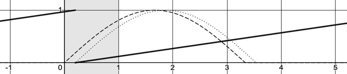
In this graph, the horizontal axis represents the passing sample frames in real-time, and the solid line is the continuous high-frequency ramp that our phasor operator is emulating. The gray-shaded region is a specific sample frame in which the phasor has wrapped, causing a trigger, and the dashed line shows a grain envelope caused by this trigger, as our patch currently produces. But for a pure tone, the grain window should be aligned to the ideal ramp, as marked by the dotted line.
We dealt with this problem previously in a somewhat ad hoc way, but it would be great if we could build a more general-purpose abstraction to extract subsample-accurate events from phasor ramp schedulers. What we need is a way to extract what the subsample offset of the ramp actually is during the trigger so that we can properly align the grain window, carrier waveform, and any other dependent processes.
There’s a simple way to calculate this: if we divide our phasor by its own slope, we’ll get a ramp with a slope of 1.0.[105] Such a slope counts by one for each passing sample frame of time. Then, in the exact sample frame that the phasor wraps, the first value will always be some number between zero and one, giving us the fractional number of samples since it wrapped (and also giving us a trigger for free).
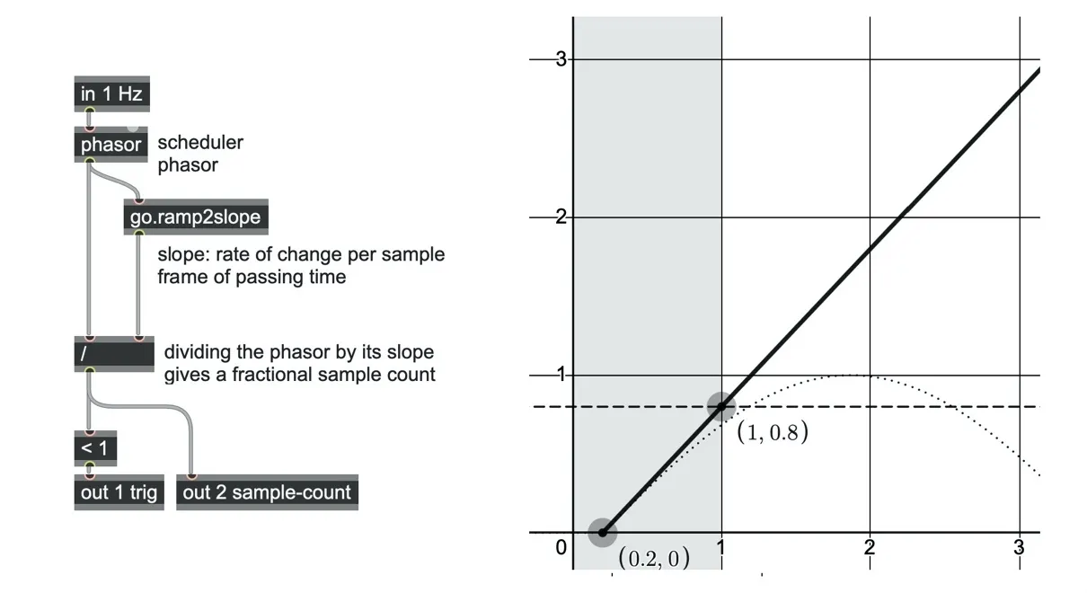
There are a few subtleties to deal with, though. First, we have to ensure we’re getting a steady rate of change of the ramp even through the transition, which we handled using the go.ramp2slope abstraction we created back in Chapter 2.
Unfortunately, this patch doesn’t work for a phasor running downwards (with negative frequency), as it will focus on the values near the top of the ramp rather than near zero. We can fix that simply by subtracting one from the phasor to recenter it, but only if the slope is negative.
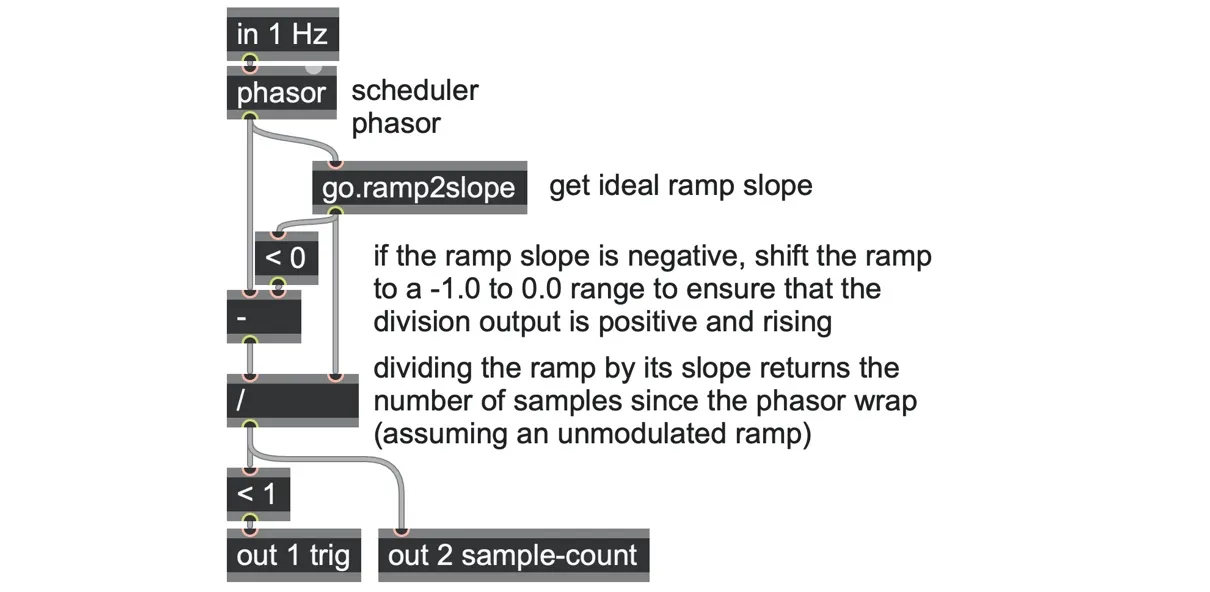
Up to now, this algorithm assumes that the phasor’s slope isn’t changing. That actually doesn’t matter for the first sample after the phasor wrap, but beyond that, simply dividing the accumulated phase by the current slope won’t accurately tell you the samples since the wrap. We can fix this easily enough by grabbing the fractional count at the wrap as we have above and storing it with a latch operator, and also restarting a sample counter using an accum 1 operator at the same time. Adding both the latch and accum 1 outputs together will give an accurate fractional measure of the number of samples since the last phasor wrap.
There’s also one more condition we might want to handle. If we ever set our phasor’s frequency to zero, then we shouldn’t be sending any triggers at all; but if we happened to do this right in the midst of a transition, the sample count might be less than one and our algorithm would be outputting triggers (and potentially spawning new grains) continuously–not at all what we want! We can fix this simply by adding a condition to the trigger that the sample count is less than one and the slope is not zero.
Here is the final patch with both of these refinements added. This is another one of those highly reusable algorithms, which we have saved as the go.ramp.subsample abstraction.
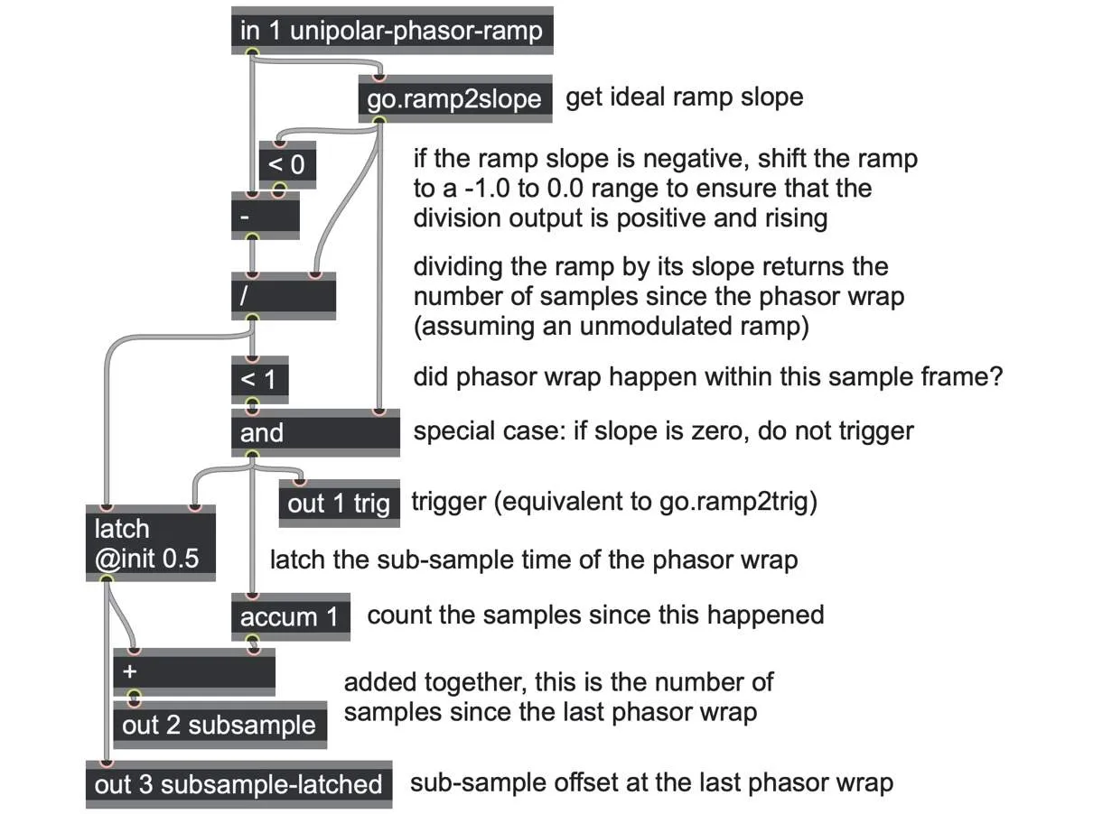
ramp-subsample-trig.maxpat and go.ramp.subsample.gendsp
We’ll be using this abstraction in the last few examples of this book, but you can see it put to use immediately in the poly_granulation3.maxpat example, where it replaces the go.ramp2trig abstraction and sends its subsample variable into a history subsample operator, ready for use in the grain3.gendsp voice subpatches.
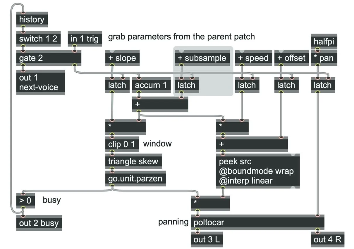
grain3.gendsp
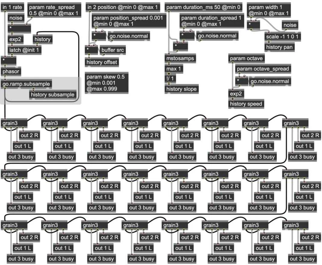
poly_granulation3.maxpat
Overdubbing the future
The strategy of passing an event on if a voice is busy works very well for overlapping events of variable durations, such as polyphonic note playing.[106] However, this strategy has a predetermined maximum polyphony (the maximum number of concurrent notes, grains, or processes). If we wanted to create very dense clouds of extremely microsonic particles, there’s an alternate strategy that might perform better, which we will explore in the next section. Before we get to that, we need to take a little detour.
If you think back to the multi-tap tape loop analogy we saw in Chapter 7, we had a single writer head, a single eraser head, and several reader heads, each of which was pulling data from the past. What if we arranged our tape loop differently, with only one reader, but instead many writers to throw sounds different distances into the future, to be heard later once the tape winds around to the reader.
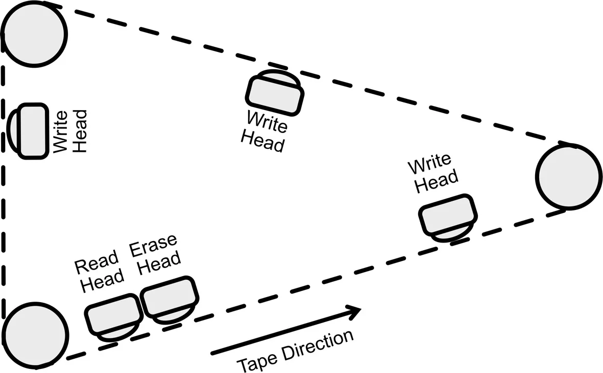
In this arrangement, the eraser head sits right after the reader to destroy sounds after they have been played. Each writer overdubs (adds) with the existing sound on the tape, accumulating many possible sound events, much like writing data into a score to be performed later. This is a kind of “overlap-add” algorithm since multiple writers can generate events that overlap with each other, and their sounds are added together.
For our tape, we can use a buffer or data operator. We’ll use a buffer operator for now so that we can visualize the contents of the tape in a Max or RNBO patch. The length of the buffer determines the maximum time that we can project sounds into the future. The tape speed is locked to real-time, moving at one sample frame of the buffer for each sample frame in real-time.
That is, at any time, the current sample index of the read head is a whole number between zero and the sample length of the buffer, and it increases by 1 for every sample frame of passing real-time, wrapping back to zero when it reaches the length of the buffer. The dim operator, or the right outlet of the buffer operator, will tell us what this length is. For the read index counter, we can use a counter operator.
The read head and eraser head are both located at this position, but we need to be careful that erasure happens after reading; a simple way is to chain the final outlet of the peek operator, which passes the sample index, into a poke operator, and write a zero to the tape at that location. This ensures that the erasure happens immediately after reading the value of the tape at that point.
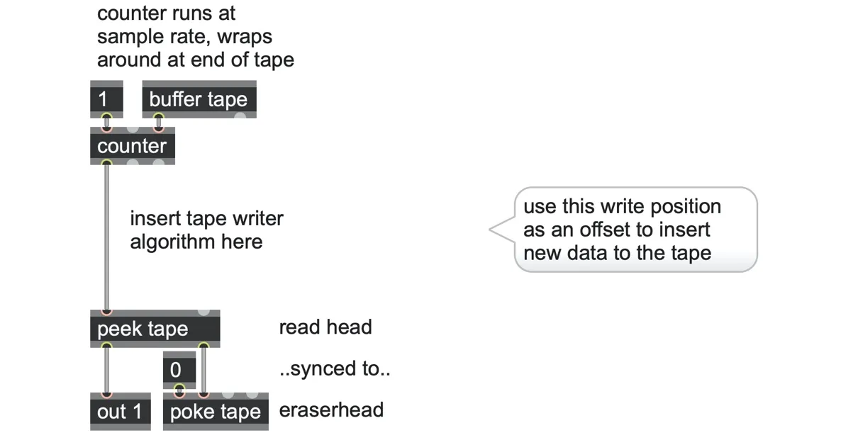
All we need to add now is one or more writer heads, using more poke operators at different positions on the tape.
Since the tape moves at 1 sample of the buffer per sample frame of real-time, then if the write head was positioned ten samples ahead of the read head (at readindex+10), we would be throwing our sound ten samples into the future, giving us a 10 sample delay between writing and reading. Similarly, for any future time N, we should write to writeindex = readindex+N.
Again we need to be careful to wrap around the tape, which poke can do automatically for us via @boundmode wrap. And, in case there’s already some data on the tape there, we will want the poke to overdub (add) rather than replace, which we can do by setting the fourth inlet’s value to one.[107]
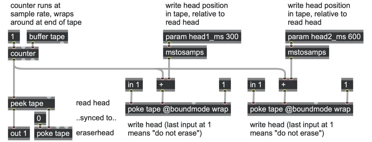
And that’s all we need to be able to throw sounds into the future. We can add as many of these write heads as we like, all writing to different places in the future, and we’ll hear the complete mix of them coming back.
There’s a catch, of course. We can’t arbitrarily modulate the delay times. If we tried to modulate the writer position N, we would end up with some probably awful noise as the incoming waveform’s samples get scattered and mixed haphazardly around the buffer tape.[108] However, we can handle sporadic stepped changes of N, and there will be no noise so long as the waveform being written is zero (or very near zero) at the moment when N changes. We can even force this to happen whenever we want by briefly “ducking” the incoming waveform. Fading it to zero, changing N, and then fading it back in. In this way, the sound being written to the tape fades to silence at the start and end of any section being written. Put another way; this means we should be windowing the source sound. This points us back toward our real reason for exploring this “future-writing strategy” as an alternative method for implementing granular synthesis.
Whole grains at once
Imagine that we had hundreds of write heads instead of just two, with each one scrubbing just a few milliseconds’ worth of enveloped sound onto the future tape at once. Hundreds of writers would mean a lot of patching, but we’ll get around this by using codebox and using a for loop to write a whole grain at a time instantaneously.
The tape playback and erasure circuit remain the same: a counter wrapping around the tape length and being fed through some algorithm that writes to the tape and then to the read head and the erase head. The actual grain generation algorithm will be written into a codebox operator sandwiched between the read counter and the reader and eraser heads. That algorithm will also need a scheduler input to know when to write a new grain.
Let’s start with a simple phasor operator running into a go.ramp2trig abstraction to turn the phasor signal into a series of triggers, routed into the codebox.
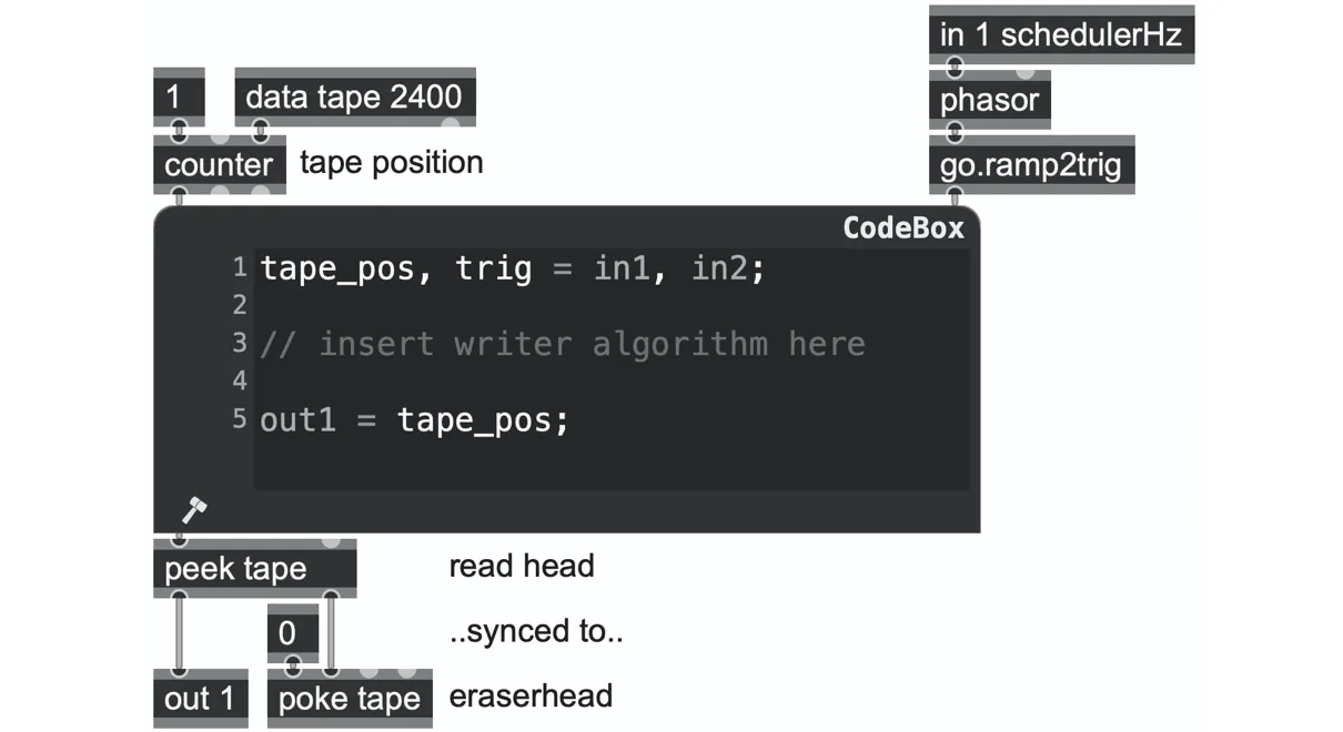
So far, this patch makes no sound, but it can be the basis for many different microsonic patches as a template. From this point on, nearly everything will happen inside the codebox. To design the algorithm, let’s start by writing pseudo-code, which just means breaking the problem into steps using plain language first to think them through and then converting these steps to real code once we have the bigger picture figured out.
First, when a trigger arrives, we want to overdub an entire grain onto the tape, all at once. In pseudo-code, the general structure is this:
if it is time to trigger a grain,
overdub an entire grain to the tape,
starting from position tape_pos
An entire grain is made up of a series of samples, which we have to generate one by one, so let’s expand that pseudo-code a little more:
if it is time to trigger a grain,
for each sample step of the grain
generate the grain’s next sample,
overdub it to the tape,
starting from position tape_pos + step
Let’s expand the grain generation. We know that grains are usually some carrier signal multiplied by some envelope signal:
if it is time to trigger a grain,
for each sample step of the grain
generate the carrier’s next sample,
generate the envelope’s next sample,
overdub carrier * envelope to the tape,
starting from position tape_pos + step
We know an envelope is a function of the grain phase, which typically runs from 0.0 to 1.0 over the length of a grain. We can get this by dividing the grain’s sample step by the grain’s length.
Let’s also start turning some of the pseudo-code into something a bit closer to GenExpr syntax:
if (trigger grain) {
for (step from zero to grain length, stepping by 1) {
phase = step / length;
envelope = something derived from phase
carrier = something
poke (carrier * envelope) to the tape
at position (tape_pos + step),
being sure to overdub,
and wrapping around the tape boundaries
}
}
That is, on each sample frame, the code will check whether it is time to generate a new grain. If so, it will use a for loop to step over each sample of the whole grain. For each step, it computes an envelope as a function of the position through the grain and uses it to multiply with a carrier sound. It overdubs the result onto the tape at the appropriate place. All of this happens within one sample frame of real-time as if the tape head whooshed by writing an entire grain onto the tape in a single instant.
Let’s fill in the remaining gaps. For now, we can set the length of the grain to 5 milliseconds, converted to sample frames:
length = mstosamps(5);
For most envelope shapes we’d need to know how far we are through a grain, which we can compute using
phase = i / length;
That will give us the envelope phase, which rises from zero to one in a straight line. We can then shape this into a triangle shape using triangle(phase) or a softer sinusoidal shape using sin(pi*phase).
env = sin(pi * phase);
For the carrier sound, we can generate a simple sine wave as a harmonic multiple of the grain period using the grain phase like this:
harmonic = 8;
carrier = sin(twopi * phase * harmonic);
Finally, we need a poke() call to write on the tape. This one has a lot of arguments corresponding to the same inlets as well as the attributes of a poke operator in a patch.
The first argument is the buffer or data to write to, which in our case is tape. Next is the value to write, which is just the carrier sound modulated by the envelope. Next is the position to write, which is the current tape head position plus the step into the grain. Next is the channel offset, which is zero since our tape is mono. The fourth argument is the amount of the original signal to preserve, which should be 1 so that the poke overdubs rather than replaces existing audio; this is the crucial argument that makes the overlap-add work. And finally, we need an attribute to make sure that if our write position is beyond the end of the tape, it wraps around back to the beginning again, via boundmode=”wrap”.
poke( tape, // the buffer or data to write to
carrier * env, // signal to write
tape_pos + step, // position on tape
0, // tape channel 0,
1, // overdub
boundmode=”wrap” ); // wrap around ends of tape
If we modify this a little bit to turn the length and harmonic values into parameters, we get the following patch, which should make a chirpy sound:
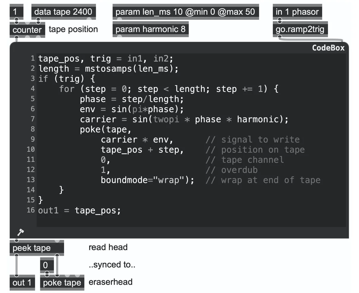
Why did we limit the param len_ms to @max 50? Because that’s as much data that can fit into our tape, that’s the longest grain the tape can support. More importantly: since the CPU has to do the work of computing the grain all at once within a single sample frame of passing time, longer grains can cause higher CPU spikes. It’s a good idea to set a limit on this to prevent audio dropouts that might happen if the CPU is too busy computing a very long grain.
The method described in this section is appropriate for microsound applications where grains are shorter than typical note lengths and more numerous than typical note polyphony. If you need to work with very long grains (approaching note lengths), this whole grain at once method probably isn’t a good approach, and the polyphonic voice method earlier in this chapter would be better.
Subsample-accurate grains
As we’ve seen before in this chapter, the subtle difference in subsample accuracy is essential for scheduling higher frequency synchronous granular synthesis. Let’s replace the go.ramp2trig with a go.ramp.subsample abstraction, which will give us the same triggers as before, as well as the subsample offsets we need. In the codebox, we will define a new variable called “subsample,” assigned from in3, and connect the abstraction’s 3rd outlet to the 3rd inlet of the codebox. We use this subsample variable to initialize step = grain_pos in the for loop. So, instead of counting from zero, our for loop will start counting from the appropriate fractional subsample location.
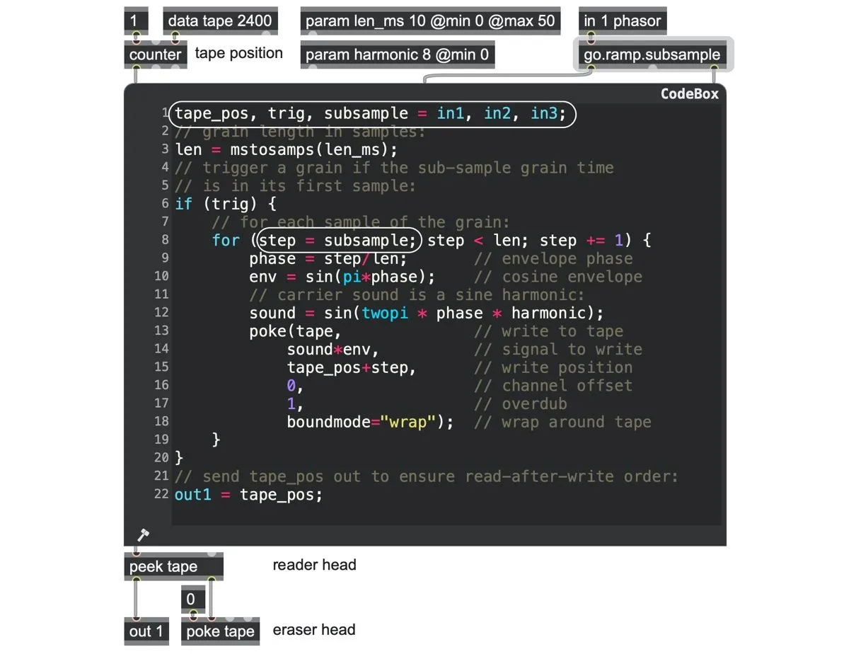
This is still a relatively simple patch, but it already pays off, especially with the intensive modulation of the phasor scheduler.
For some much more involved examples, you can look at the granola patches in the book’s software package, which extend this patch with additional parameters and different carrier waveforms. The granola_buffer.maxpat example demonstrates reading from a buffer in a similar way to the polyphonic granulation example earlier in this chapter. The granola_glisson.maxpat demonstrates a more complex synthesized waveform in the form of “glisson synthesis”, where each grain is a glissando from one pitch to another.
A bandlimited saw with hard sync
As a final example of the importance of thinking in subsample times, let’s circle back to that challenge we raised at the start of this chapter: how to produce waveforms with hard cuts like sawtooth shapes (and pitched phasors), as well as general hard sync effects, without causing unpleasant aliasing noise. There are plenty of different approaches to creating bandlimited oscillators, including using oversampling, using bandlimited impulse trains (BLIT), bandlimited steps (“BLEPs”), etc., with various benefits and trade-offs that we will delve into in Book 2. But to close this chapter, we’re going to describe a different method that performs remarkably well for how cheap and flexible it is.[109]
This is a somewhat subtle patch, so it’s going to be helpful to understand what it solves and why it works before we start to build it. Let’s start back at the beginning with a classic phasor ramp, whose ideal, continuous form looks like this:
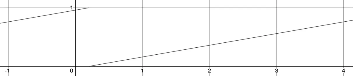
That graph is ideal because it is continuous, with infinite resolution. In practice, we only have the resolution of the sample rate, so, zoomed into the level of the sample frames, our typical phasor algorithm approximates the ideal graph by stepping with each sample frame, like the dashed lines here:
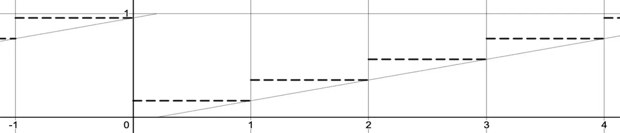
But there’s no way that an actual loudspeaker’s diaphragm can instantaneously jump from one position to another like this—it has to move continuously, just like an interpolation. The simplest imaginable path without instantaneous jumps is a straight line between each sample, like the dotted path below:[110]
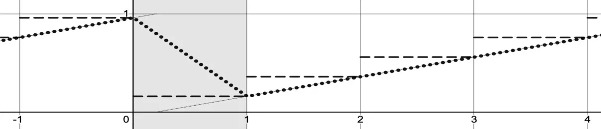
Compared to the ideal phasor, we can see that it diverges for exactly the one sample where the transition occurs (which we have shaded in gray). Everything that we are going to do is focused on changing this one sample frame.
Take a closer look at the values of the phasor where it enters and exits the gray region. You’ll notice that these points are not symmetric: it enters very close to 1.0, but when it exits, it isn’t nearly so close to 0.0; that’s because the transition itself doesn’t align perfectly with the sampling rate. That slight deviation might not seem like much, but over many cycles of the phasor, it can add up to a big sonic difference.
To make this visually very obvious, in the following graph we have set the phasor frequency much higher:
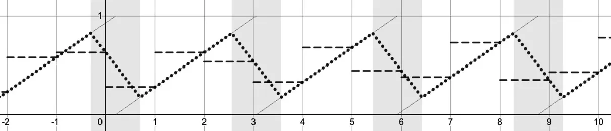
You can clearly see that with each gray-shaded transition sample, the apparent phasor (dotted line) that joins up our sample values enters and exits at quite different positions, creating an impression of irregular harmonic periods. These divergences thus introduce unrelated audible frequencies into the sound of the phasor, which is a form of digital aliasing noise.
The good news is that with these observations, we already have everything we need to solve the problem.
We know that we can’t actually render an instantaneous jump of the phasor; we must instead always have a sloping line of (at least) one sample’s duration.
We know that aliasing occurs because the ramp values during a transition depend on the relative alignment of the phasor wrap with the sampling rate, not the timing of the phasor itself.
So, what if, instead of trying to synthesize an impossible ideal phasor, we synthesize a function that already has the single-sample slope requirement embedded into it? And, to make this independent of the sampling points, what if we place that slope precisely centered on the ideal phasor’s transition point rather than the sampling grid?
That is, if we try to synthesize this waveform:
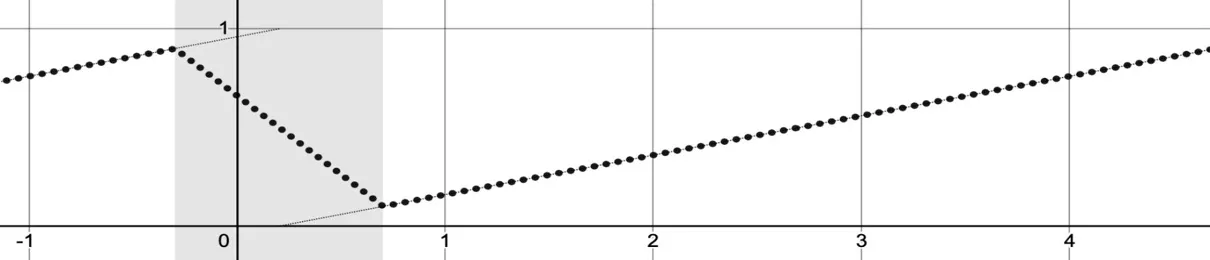
Notice that the dotted path is still exactly the same as the ideal phasor outside of the gray zone. The gray region of the transition sample is no longer aligned to the sample points but is instead exactly centered on the phasor’s ideal transition. The entry and exit points of the gray zone are always symmetric.
Even at the same high frequency we used earlier, this waveform remains regular and balanced. And since no slope is ever steeper than what can be achieved in a single sample frame, this waveform can be rendered in digital samples without creating lots of aliasing.

The gray zone itself is still only one sample frame long, which means that there’s only one sample we need to change. And all we need to know to compute that change is the following information:
The phasor value at the entry and exit points of the gray region exactly half a sample before and after the ideal transition. These points define the start and end of the single-sample downward ramp of the transition.
The subsample position where the transition occurs so that we can extract the value of that downward ramp in the right place.
Time to get patching! We can start from the non-antialiased phasor we have seen since the start of this book:

We want to know the values of the ideal ramp that this phasor represents, one-half a sample frame before and after it has a transition. The value half of a sample after a transition is pretty simple: since the phasor rises by a known slope for each sample frame, then half a sample frame after it wraps it will have risen by slope * 0.5. Except if the ramp is running in reverse; in that case, it will have fallen to 1.0 - (slope * 0.5). Then the value of the phasor one-half of a sample before a transition is just the mirror of the state half a sample after.
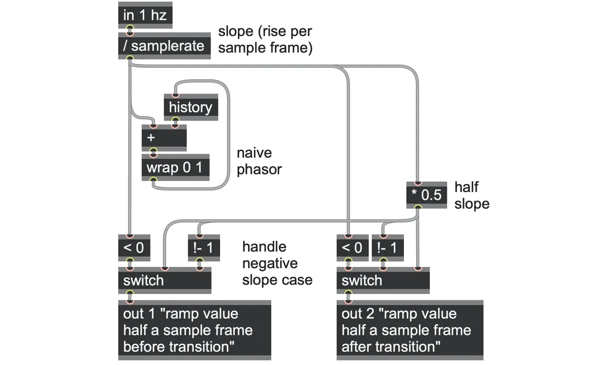
So, for example, if the phasor frequency is equal to samplerate/5, then the ramp value half a sample before a transition is 0.9, and the ramp value half a sample after a transition is 0.1. These are the highest and lowest values our antialiased phasor can reach and the entry and exit corner points of the gray region.
All we need to know now is the subsample location (i.e., the fractional sample count) of the ideal transition relative to our sampling grid so that we can get the value of the ramp between these two corner points. As we learned with the subsample ramp trigger in the granular scheduler, we can get the fractional sample count of a ramp by dividing the ramp’s value by its slope.
To handle both rising and falling ramps, we can first recenter the phasor in the -0.5 to 0.5 range. Then we project half a sample ahead (by adding half a slope) to get our transition point and then divide by the slope. That will give us the fractional sample count of up to half a sample before or after the ideal transition.
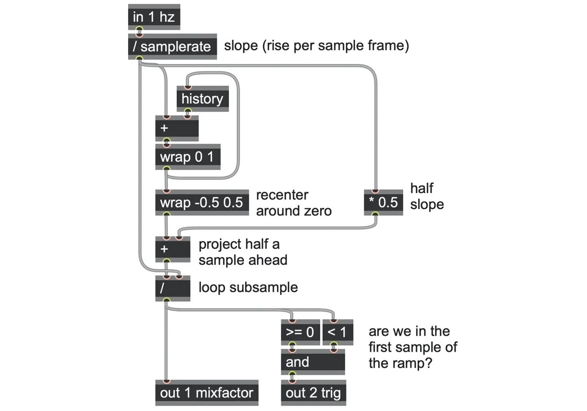
As a bonus, we can also use this fractional sample count as our trigger detection, just as we did with the go.ramp.subsample abstraction. Simply: if we are in the first sample frame of a phasor’s ramp, then the fractional sample count will be between zero and one, which means we are in the gray zone, and we can output a trigger when that happens.
Now we can put everything together. When we are in the gray zone (i.e., the trigger fires at out 2), we want to replace the basic aliasing phasor with a new value that is taken instead from a replacement ramp between the entry and exit points of the gray region. We can use switch operators to swap in these values when the trigger happens.
And since the replacement ramp we are inserting is linear, we can simply crossfade between them using a mix operator, using the fractional subsample time as the crossfade factor.
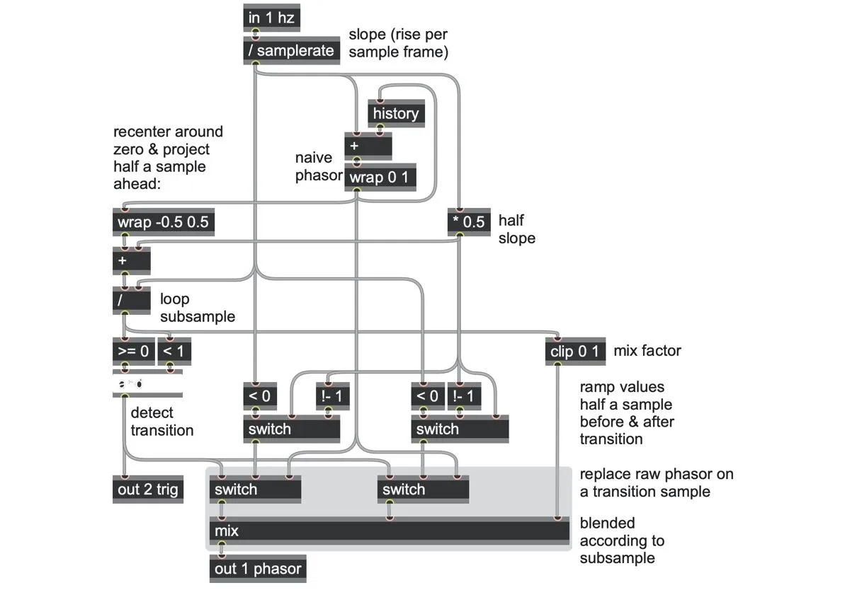
And that gives us exactly the output of the sampled antialiased waveform we wanted! It results in a unipolar ramp with far less aliasing than a phasor operator, with no latency, and at very little computational expense.
The following spectrum shows both—the standard phasor operator in gray and our antialiased phasor here in black - running at around 2500Hz.

You can immediately see how the black spectrum has a clearly defined shape with far fewer aliasing harmonics than the gray, aliasing phasor. The principal harmonics hold their strength well going up the spectrum, keeping the brightness of the sawtooth sound present, but the aliasing harmonics fall quickly to zero on the first reflection back and are practically inaudible, whereas the gray basic phasor continues to produce aliasing frequencies reflecting several times over the spectrum. It’s not perfect antialiasing, but it is remarkably practical and effective for its simplicity.[111] It can also handle deep frequency modulation and, as we shall see, can be extended to support hard sync and some wave shaping. It all came down to creating a waveform in which no slope is sharper than a single sample and aligning those transitions to the ideal shape of the waveform rather than to the sampling grid.
Adding hard sync
First, we will need another oscillator as the hard sync source. With analog synthesizers, that would typically be some kind of trigger generator, but we will work with another phasor ramp here. Why? As we have seen throughout this chapter, it becomes essential to think about fractional sample counts and subsample accuracy for pitched oscillators, and hard sync is no exception. When a hard sync phasor reset happens, does it happen at the start of a sample frame, at the end, or somewhere in between? To specify that kind of accuracy, we can’t rely on trigger signals alone.
Instead, here we are going to reuse the subsample-accurate ramp transition detector we built earlier in this chapter as the go.ramp.subsample abstraction. The first outlet of this abstraction gives a trigger when a transition occurs, while the 3rd outlet gives us the fractional offset of that transition within a sample frame. So, for the raw (aliasing) synced phasor, we can insert a switch operator to reset the phase when the go.ramp.subsample trigger occurs, and the value we reset it to is the subsample offset multiplied by the slope.
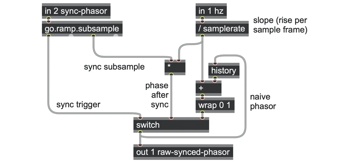
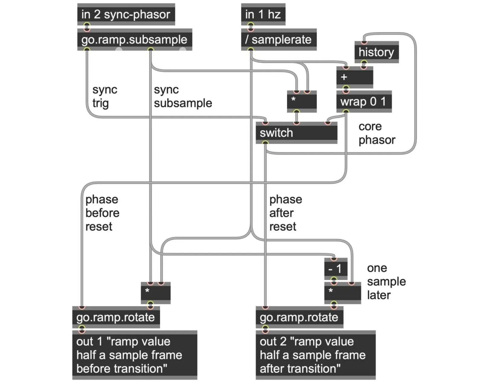
That subsample offset will also stand in as our mix factor for the antialiasing mix operator when a sync trigger occurs. But first, we need to compute the ramp phases half a sample before and after the sync event. This is a little more complex now since a sync event could happen anywhere during the ramp’s progress. But we can figure it out by working back from the current ramp’s value (before the reset) or forward (after the reset) by reusing our go.ramp.rotate abstraction from Chapter 2, and using the subsample offset multiplied by the slope to know how far to rotate:
Now we just need to integrate these revisions with our antialiased phasor. This is mostly just careful plumbing and the insertion of a switch operator to select between the subsample offset of a normal phasor wrap transition versus a hard sync transition:
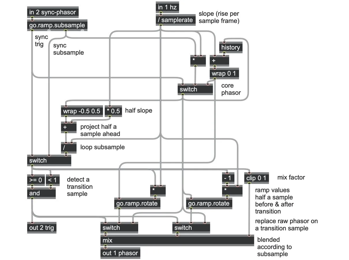
go.ramp.aa
And that gives us a very reliable antialiased phasor ramp that supports subsample accurate hard sync as well as deep frequency modulation, both up to audio rates!
Shaping
There’s one more neat thing we can do with this patch. We can apply some unit shaping curvatures to the signals between the mix operator and the switch operators at the bottom of the patch. So long as the unit shapes start at 0.0, end at 1.0 and have no sharp cuts of their own, then the output of the patch will remain pretty well antialiased.
Some examples of unit shapers you can try here include go.unit.arc2, go.unit.triangle, go.unit.tukey, go.unit.cubic, go.unit.ease.exp, go.unit.ease.sine, etc. The ramp_antialiased.maxpat patch shows an example of chaining two unit shapers for a relatively complex waveform. Here are some example shapes (with the transition and sync triggers overlaid in gray), along with the corresponding aliased (gray) and antialiased (black) spectra:
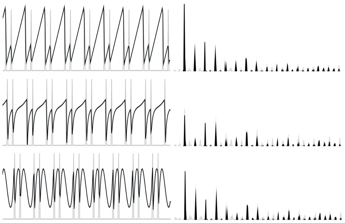
Here are a few more example waveforms and spectra using deep through-zero frequency modulation, including the ramp itself, as well as the ramp providing the hard sync signal, which this patch handles very well: 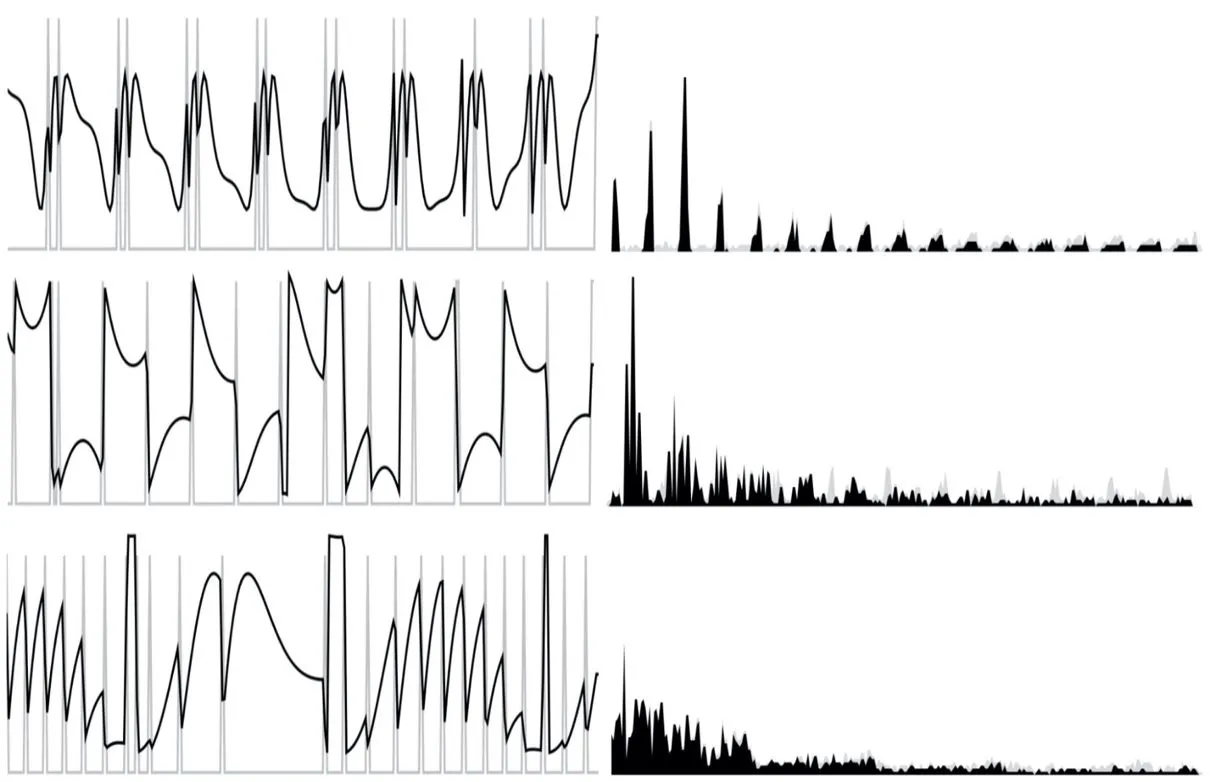
Naturally, you can try substituting this oscillator into some of the FM structures we encountered in Chapter 8 or perhaps with some of the ramp division modulations we met at the end of Chapter 2.